The Deadly Triad
Revised December 16, 2024
The Off-Policy Control with Function Approximation note is optional but recommended background reading.
The deadly triad refers to the instability — that is, the risk of divergence — that can arise when combining off-policy training, function approximation, and bootstrapping. All known divergence examples for TD-style methods involve all three components; standard algorithms using only two (e.g., tabular off-policy TD, or on-policy TD with function approximation) are typically stable. However, when all three are combined, instability can emerge in both prediction and control tasks. This risk of divergence is not inherent to the learning process itself or caused by environmental uncertainty; it can also occur in planning methods, such as approximate dynamic programming, where the environment is fully known.
The deadly triad affects only semi-gradient methods; true gradient methods are immune. Despite this theoretical advantage, true gradient methods are less commonly used in practice than semi-gradient methods, making the risks associated with the deadly triad particularly relevant. Baird's counterexample is a well-known illustration of this instability.
Consider an episodic six-state MDP with two actions. Five of the states are nonterminal (the upper states) and one is terminal (the lower state). The dashed action selects one of the five upper states with equal probability. The solid action transitions directly to the terminal state. Under the behavior policy \(\pi_\beta\), the dashed and solid actions are chosen with probabilities \(\tfrac{5}{6}\) and \(\tfrac{1}{6}\), respectively, resulting in a uniform next-state distribution over the nonterminal states. This same distribution is used to initialize each episode. The target policy \(\pi\) always selects the solid action, so its stationary distribution places all probability on the terminal state. All rewards are zero (so the true value function is \(V_*(s) = 0 \; \forall s\)), and the discount factor is \(\gamma = 0.99\).
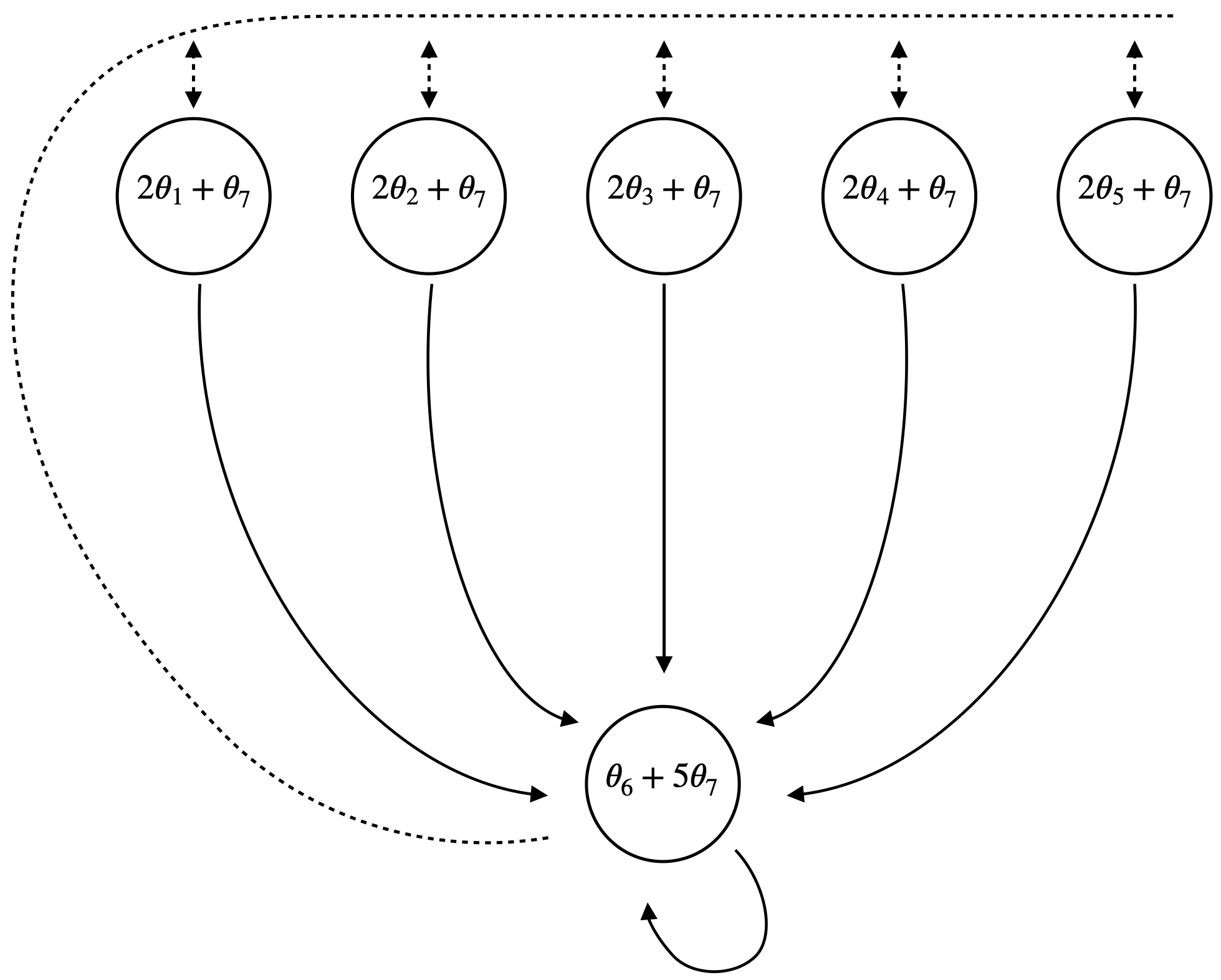 |
Suppose the value of each state is estimated as a linear combination of parameters. For instance, the estimated value of state \(s_1\) is given by \(2\theta_1 + \theta_7\), where \(\theta_1\) and \(\theta_7\) are components of the parameter vector \(\theta \in \mathbb{R}^7\). The corresponding feature vector for \(s_1\) is \(\phi_{s_1} = [2, 0, 0, 0, 0, 0, 1]^\top\).
The feature vectors for all states can be organized into a matrix \(\Phi\), wherein each row corresponds to the feature vector of a specific state. This matrix representation facilitates operations on the entire set of states (as was seen, for example, when using the projection operator):
\[ \begin{equation*} \Phi = \begin{bmatrix} 2 & 0 & 0 & 0 & 0 & 0 & 1 \\ 0 & 2 & 0 & 0 & 0 & 0 & 1 \\ 0 & 0 & 2 & 0 & 0 & 0 & 1 \\ 0 & 0 & 0 & 2 & 0 & 0 & 1 \\ 0 & 0 & 0 & 0 & 2 & 0 & 1 \\ 0 & 0 & 0 & 0 & 0 & 1 & 5 \\ \end{bmatrix} \end{equation*} \]
Using \(\Phi\), the true value function \(V_* = 0\) can be represented exactly as \(V_* = \Phi \theta\) by setting \(\theta = 0\):
\[ \begin{equation*} \hat{V} = \begin{bmatrix} 2 & 0 & 0 & 0 & 0 & 0 & 1 \\ 0 & 2 & 0 & 0 & 0 & 0 & 1 \\ 0 & 0 & 2 & 0 & 0 & 0 & 1 \\ 0 & 0 & 0 & 2 & 0 & 0 & 1 \\ 0 & 0 & 0 & 0 & 2 & 0 & 1 \\ 0 & 0 & 0 & 0 & 0 & 1 & 5 \end{bmatrix} \begin{bmatrix} 0 \\ 0 \\ 0 \\ 0 \\ 0 \\ 0 \\ 0 \end{bmatrix} = \begin{bmatrix} 0 \\ 0 \\ 0 \\ 0 \\ 0 \\ 0 \end{bmatrix} \end{equation*} \]
Notably, there are infinitely many choices for \(\theta\) such that \(\Phi \theta = 0\). For instance, consider \(\theta = [\frac{1}{2}, \frac{1}{2}, \frac{1}{2}, \frac{1}{2}, \frac{1}{2}, 5, -1 ]^\top\):
\[ \begin{equation*} \hat{V} = \begin{bmatrix} 2 & 0 & 0 & 0 & 0 & 0 & 1 \\ 0 & 2 & 0 & 0 & 0 & 0 & 1 \\ 0 & 0 & 2 & 0 & 0 & 0 & 1 \\ 0 & 0 & 0 & 2 & 0 & 0 & 1 \\ 0 & 0 & 0 & 0 & 2 & 0 & 1 \\ 0 & 0 & 0 & 0 & 0 & 1 & 5 \end{bmatrix} \begin{bmatrix} \frac{1}{2} \\ \frac{1}{2} \\ \frac{1}{2} \\ \frac{1}{2} \\ \frac{1}{2} \\ 5 \\ -1 \end{bmatrix} = \begin{bmatrix} 0 \\ 0 \\ 0 \\ 0 \\ 0 \\ 0 \end{bmatrix} \;. \end{equation*} \]
In fact, the vector \(\theta = [\frac{1}{2}, \frac{1}{2}, \frac{1}{2}, \frac{1}{2}, \frac{1}{2}, 5, -1 ]^\top\) lies in the null space of \(\Phi\), meaning any scalar multiple of \(\theta\) will also satisfy \(\Phi \theta = 0\). This observation, combined with the linear independence of the feature vectors, suggests that learning a linear approximation using a semi-gradient method should, in principle, be straightforward. However, we observe that the parameters diverge to infinity when the semi-gradient TD(0) update rule is applied:
\[ \begin{equation*} \theta \gets \theta + \alpha \left[ r + \gamma \hat{V}(s’; \theta) - \hat{V} (s; \theta) \right] \nabla \hat{V}(s; \theta) \;. \end{equation*} \]
Let the initial parameters be \(\theta_i = 1\) for all \(i\). With this initialization, \(\hat{V}(s_1) = 3\) and \(\hat{V}(s_6) = 6\). Now, suppose we observe a transition from \(s_1\) to \(s_6\) at time \(t\). Then, assuming a discount factor \(\gamma = 0.99\) and step size \(\alpha = 0.1\), the temporal difference (TD) error \(\delta\) is calculated as:
\[ \begin{equation*} \delta = r + \gamma \hat{V}(s_6) - \hat{V}(s_1) = 0 + 0.99 \cdot 6 - 3 = 2.94. \end{equation*} \]
Since \(\hat{V}(s_1) = 2\theta_1 + \theta_7\), the gradients of \(\hat{V}(s_1)\) with respect to the parameters are:
\[ \begin{equation*} \frac{\partial \hat{V}(s_1)}{\partial \theta_1} = 2 \quad \text{and} \quad \frac{\partial \hat{V}(s_1)}{\partial \theta_7} = 1. \end{equation*} \]
Using these gradients, the updates to \(\theta_1 = 1\) and \(\theta_7 = 1\) are:
\[ \begin{align*} \theta_1 &\gets \theta_1 + (\alpha \delta)2 = 1 + 0.1 \cdot 2.94 \cdot 2 = 1.588, \\ \theta_7 &\gets \theta_7 + \alpha \delta = 1 + 0.1 \cdot 2.94 \cdot 1 = 1.294. \end{align*} \]
If we compute the update for each step from states \(s_1\) through \(s_5\) to \(s_6\), we find that \(\theta_7\) increases with every iteration:
\[ \begin{align*} s_1 \rightarrow s_6: \theta_7 &= 1.294 \\ s_2 \rightarrow s_6: \theta_7 &= 1.704 \\ s_3 \rightarrow s_6: \theta_7 &= 2.276 \\ s_4 \rightarrow s_6: \theta_7 &= 3.074 \\ s_5 \rightarrow s_6: \theta_7 &= 4.188 \;. \end{align*} \]
Therefore, steps from \(s_6\) to itself must reduce \(\theta_7\); otherwise, the parameters \(\theta_i\) will grow without bound. To quantify the impact of a step from \(s_6\) to itself on \(\theta_7\), we calculate the corresponding update:
\[ \begin{equation*} \theta_7 = 4.188 + 0.1 \Big[ 0 + 0.99 \cdot \big( 1 + (5 \cdot 4.188) \big) - \big( 1 + (5 \cdot 4.188) \big) \Big] \cdot 5 = 4.0783 \;. \end{equation*} \]
Although this update reduces \(\theta_7\), the reduction is small: \(4.188 - 4.0783 = 0.1097\). As illustrated in the figure below, this reduction is insufficient to mitigate the overall growth of the parameters, leading to instability.
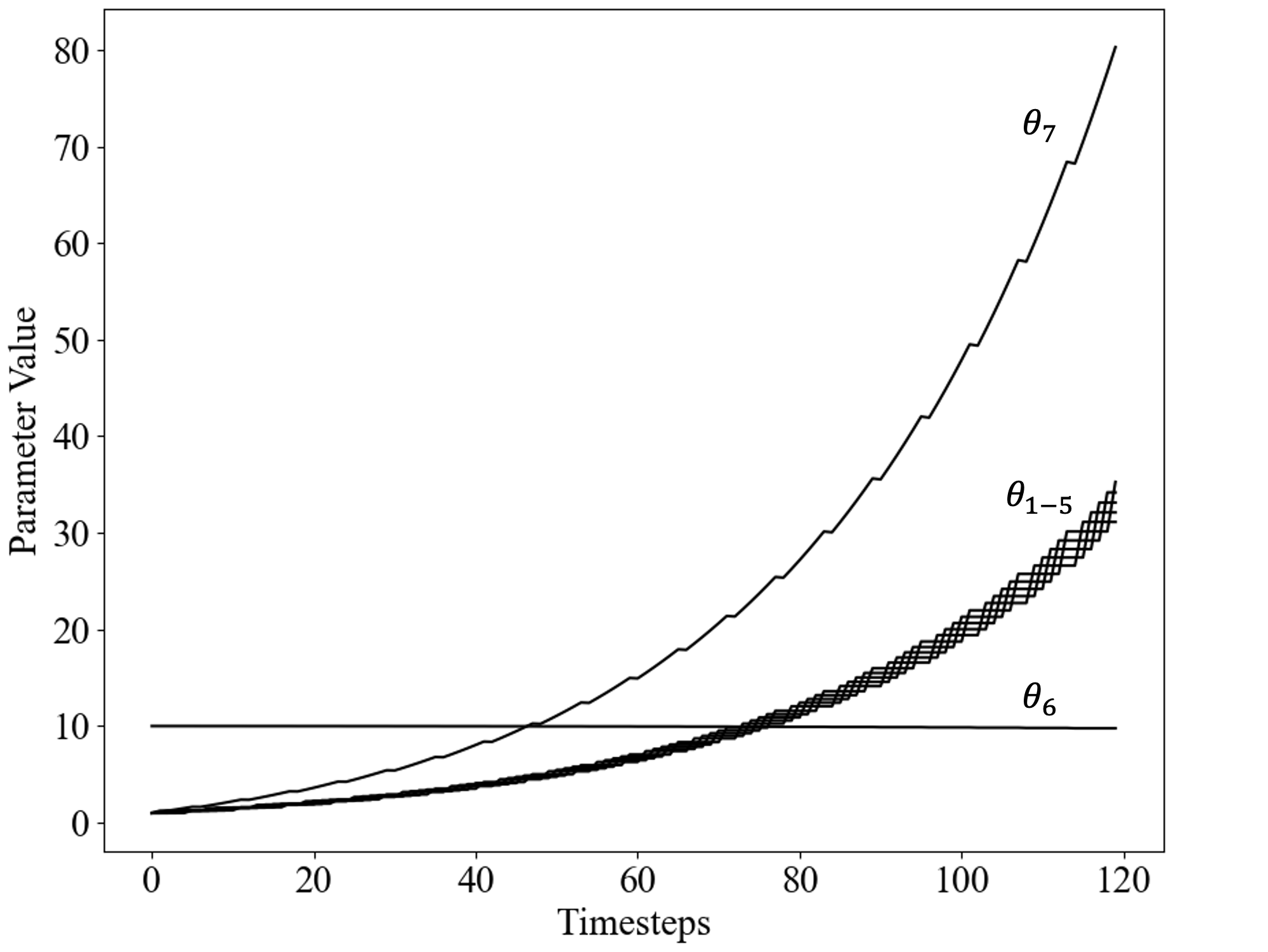 |
| Results computed with step size \(\alpha = 0.01\), \(\gamma = 0.99\), and initial parameters \(\theta = [1, 1, 1, 1, 1, 10, 1]^\top\). |
There are also counterexamples, similar to Baird’s, demonstrating divergence in Q-learning. However, the conditions under which divergence occurs are not well understood. This is particularly concerning because Q-learning otherwise provides the strongest convergence guarantees among control methods and serves as the foundation for many modern RL algorithms, such as deep Q-learning. Significant effort has been devoted to addressing this issue or establishing weaker but practical convergence guarantees. For instance, although standard deep Q-learning lacks formal convergence guarantees, some results have been obtained for a related algorithm, Neural-Fitted Q Iteration, when combined with deep ReLU networks. Moreover, convergence in Q-learning may still be achievable if the behavior policy is sufficiently close to the target policy, as in the case of an \(\epsilon\)-greedy policy.
Citation
Landers, Matthew. "The Deadly Triad." mattlanders.net, December 16, 2024. mattlanders.net/the-deadly-triad.
@article{landers2024deadly,
  title = {The Deadly Triad},
  author = {Landers, Matthew},
  journal = {mattlanders.net},
  year = {2024},
  month = {December},
  url = "mattlanders.net/the-deadly-triad"
}
References
- Reinforcement Learning: An Introduction (2018)
Richard S. Sutton and Andrew G. Barto
- Introduction to Reinforcement Learning with Function Approximation (1995)
Richard S. Sutton
- Deep Reinforcement Learning [video]
Charles Isbell, Michael Littman, and Chris Pryby
- Towards Characterizing Divergence in Deep Q-Learning (2019)
Joshua Achiam, Ethan Knight, and Pieter Abbeel
- A Theoretical Analysis of Deep Q-Learning (2020)
Jianqing Fan, Zhaoran Wang, Yuchen Xie, and Zhuoran Yang