The Learnability of RL Objectives
Revised December 12, 2024
The Prediction with Function Approximation and Off-Policy Control with Function Approximation notes are optional but recommended background reading.
When a policy's true value function, \(V_\pi\) (or \(Q_\pi\)), is too complex to learn exactly, it can be approximated using a parameterized function \(\hat{V}(\theta)\) (or \(\hat{Q}(\theta)\)). The optimal approximation is found by iteratively adjusting parameters \(\theta\) to minimize a chosen error criterion, measured using a norm. While many error criteria exist, RL methods typically use a select few. This note examines the “learnability” of such error criteria. In general machine learning literature, learnability refers to the ability to minimize an error function to an arbitrarily small value from a finite number of samples. Here, we adopt a broader notion of learnability to examine whether an error criterion can be minimized to arbitrary precision, even when given an infinite number of samples.
We begin by defining the error criteria under consideration. Most of these definitions come from the prediction with function approximation and off-policy control with function approximation notes, where additional context is provided but learnability is not addressed.
Monte Carlo Objectives
Because convergence to a local optimum is guaranteed only when using an unbiased estimator, Monte Carlo (MC) and bootstrapping methods use different objective functions. We begin with the MC error criteria.
Value Error
Our goal is to find an approximation \(\hat{V}(\theta)\) that closely matches the true value function \(V_\pi\). Thus, minimizing the mean squared error (MSE) between \(V_\pi\) and \(\hat{V}(\theta)\) is a natural objective. This error is quantified using a weighted Euclidean norm:
\[ \begin{equation}\label{eq:value_error} \overline{\text{VE}}(\theta) = \sum_{s \in \mathcal{S}} \mu(s) \left[V_\pi(s) - \hat{V}(s; \theta) \right]^2 \;, \end{equation} \]
where \(\mu(s)\) is a state distribution satisfying \(\sum_s \mu(s) = 1\) and \(\theta\) is a parameter vector with \(|\theta| < |\mathcal{S}|\). The distribution \(\mu(s)\) weights each state's error contribution, reflecting the need to prioritize minimizing errors in certain states, as it is generally impossible to reduce error to zero across all states.
This loss can also be expressed using the following norm:
\[ \begin{equation}\label{eq:squared-norm-of-vector} \| f \|_\mu^2 = \sum_{s \in \mathcal{S}} \mu(s) f(s)^2 \;. \end{equation} \]
It represents the “length” or magnitude of an arbitrary function \(f\), weighted by \(\mu\). Using this formulation, the mean squared value error can be written as \(\overline{\text{VE}} = \| \hat{V}(\theta) - V_\pi \|_\mu^2\).
Return Error
Given the value function estimates returns, it is also reasonable to minimize mean square return error. This error is defined as the expectation, under the distribution \(\mu\), of the squared difference between the estimated value function \(\hat{V}(\theta)\) at time step \(t\) and the actual return \(G_t\). For the on-policy case, this objective can be expressed as:
\[ \begin{align} \overline{\text{RE}}(\theta) &= \mathbb{E}_{s \sim \mu} \left[ \mathbb{E} \left[ \left( G_t - \hat{V}(s; \theta) \right)^2 \mid s_t = s \right] \right] \nonumber \\ &= \sum_{s \in \mathcal{S}} \mu(s) \mathbb{E} \left[ \left( G_t - \hat{V}(s; \theta) \right)^2 \mid s_t = s \right] \nonumber \\ &= \sum_{s \in \mathcal{S}} \mu(s) \mathbb{E} \left[ \left( \left( G_t - V_\pi(s) \right) + \left( V_\pi(s) - \hat{V}(s; \theta) \right) \right)^2 \mid s_t = s \right] \nonumber \\ &= \sum_{s \in \mathcal{S}} \mu(s) \mathbb{E} \left[ \left( G_t - V_\pi(s) \right)^2 + \left( V_\pi(s) - \hat{V}(s; \theta) \right)^2 + 2 \left( G_t - V_\pi(s) \right) \left( V_\pi(s) - \hat{V}(s; \theta) \right) \Bigg| s_t = s \right] \nonumber \\ &= \sum_{s \in \mathcal{S}} \mu(s) \left[ \mathbb{E} \left[ \left( G_t - V_\pi(s) \right)^2 \mid s_t = s \right] + \left( V_\pi(s) - \hat{V}(s; \theta) \right)^2 + 2 \left( V_\pi(s) - \hat{V}(s; \theta) \right) \mathbb{E} \left[ G_t - V_\pi(s) \mid s_t = s \right] \right] \nonumber \\ &= \sum_{s \in \mathcal{S}} \mu(s) \left[ \mathbb{E} \left[ \left( G_t - V_\pi(s) \right)^2 \mid s_t = s \right] + \left( V_\pi(s) - \hat{V}(s; \theta) \right)^2 + 2 \left( V_\pi(s) - \hat{V}(s; \theta) \right) \times 0 \right] \nonumber \\ &= \sum_{s \in \mathcal{S}} \mu(s) \left[ \left( V_\pi(s) - \hat{V}(s; \theta) \right)^2 \right] + \sum_{s \in \mathcal{S}} \mu(s) \mathbb{E} \left[ \left( G_t - V_\pi(s) \right)^2 \mid s_t = s \right] \nonumber \\ &= \overline{\text{VE}}(\theta) + \mathbb{E} \left[ \left( G_t - V_\pi(s_t) \right)^2 \right] \;. \label{eq:re-8} \\ \end{align} \]
Starting from the definition of the return error, we begin with the expectation under the behavior distribution \(\mu\) of the squared difference between the return \(G_t\) and the approximate value \(\hat{V}(s;\theta)\). First, we explicitly write out the expectation over states as a sum over all states weighted by \(\mu(s)\). Next, we add and subtract the true value function \(V_\pi(s)\) inside the square, which allows us to separate the deviation \(G_t - \hat{V}(s;\theta)\) into two parts: the “intrinsic noise” \(G_t - V_\pi(s)\) and the approximation error \(V_\pi(s) - \hat{V}(s;\theta)\). Squaring this sum and expanding it, we get three terms: the variance term \((G_t - V_\pi(s))^2\), the approximation error \((V_\pi(s) - \hat{V}(s;\theta))^2\), and a cross term involving the expectation of \((G_t - V_\pi(s))\). Because \(G_t\) is an unbiased estimator of \(V_\pi(s)\), that cross term vanishes, reducing the expression. This simplifies the return error into a sum of two parts: the value error, which is the weighted expectation of \((V_\pi(s) - \hat{V}(s;\theta))^2\), and the irreducible error from the return variance \(\mathbb{E}[(G_t - V_\pi(s_t))^2]\).
The Learnability of MC Objectives
To evaluate whether value error and return error are “learnable”, we must first define what it means for an error to be “learnable.” This concept can be most simply illustrated using an example based on the mean squared value error (Equation \(\eqref{eq:value_error}\)).
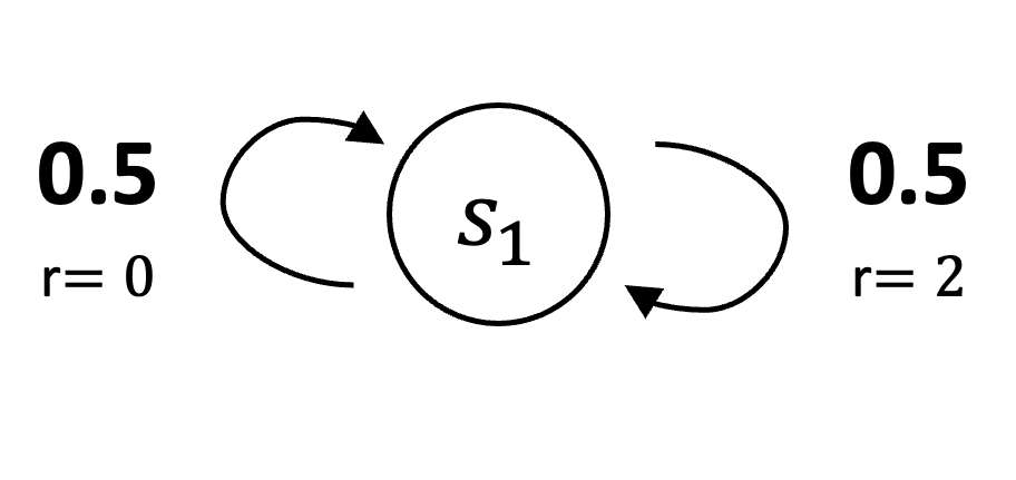
Consider a one-state Markov reward process (MRP) in which the agent always transitions back to the same state, \(s_1\). The reward for this transition is stochastic: with probability \(0.5\), the reward is \(0\), and with probability \(0.5\), the reward is \(2\). The state, \(s_1\), is represented by a single-component feature vector \(\phi = 1\) and has an approximate value \(\theta\). Consequently, the only varying component of the data trajectory is the reward sequence — a random stream of \(0\)s and \(2\)s.
 |
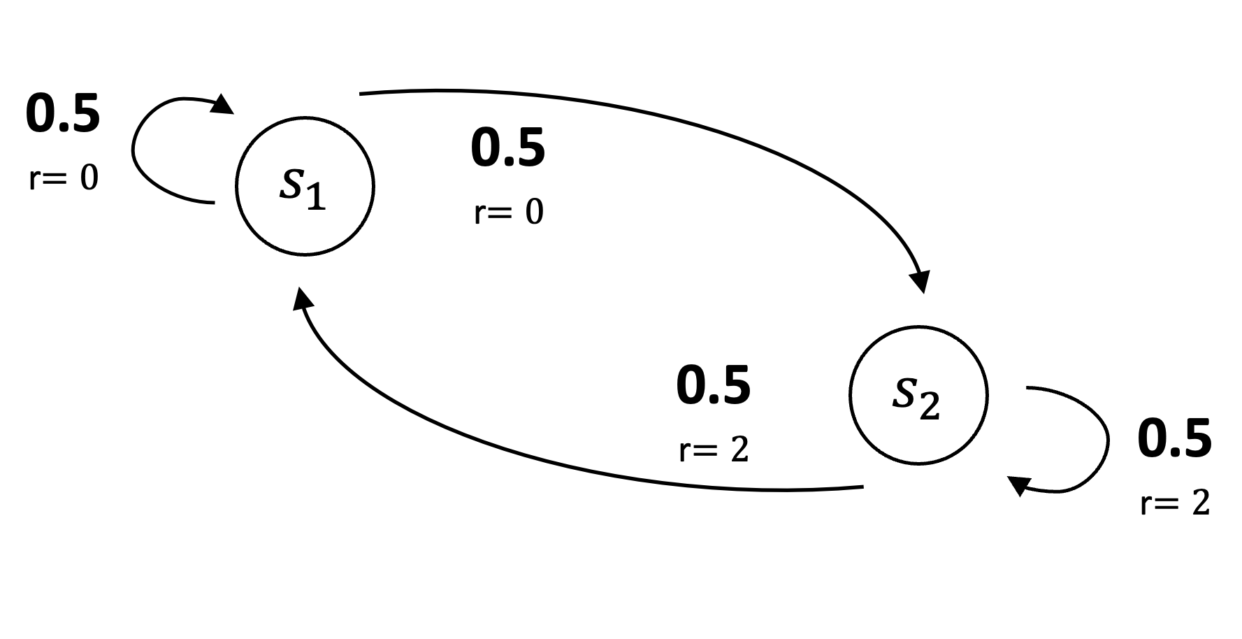
Now consider a two-state MRP in which the agent transitions from state \(s_1\) to \(s_2\) with probability \(0.5\) and back to \(s_1\) with probability \(0.5\). Unlike the first MRP, the rewards for these transitions are deterministic, with both yielding a reward of \(0\). From state \(s_2\), the agent transitions to \(s_1\) with probability \(0.5\) and remains in \(s_2\) with probability \(0.5\). The reward for these transitions are also deterministic, both yield a reward of \(2\). As in the first MRP, both states are represented by a single-component feature vector \(\phi = 1\) and have an approximate value \(\theta\). Similarly, the only varying component of the data trajectory is the reward sequence, which is an endless random stream of \(0\)s and \(2\)s.
 |
Even though the reward sequences in these two systems may differ in order, the probabilities of observing \(0\)s and \(2\)s are identical. Consequently, the data trajectory provides no signal to distinguish which MRP is generating the data. In particular, we cannot determine whether the MRP has one state or two, or whether its dynamics are stochastic or deterministic. While it would be possible to differentiate the MRPs if we observed the states directly, the use of function approximation means we only observe feature vectors \(\phi\), which are also identical.
These MRPs also illustrate that \(\overline{\text{VE}}\) cannot be learned.
Assume \(\gamma = 0\). In the first MRP, the true value of \(s_1\) is the mean reward, which is \(1\). If \(\theta = 1\) and \(\phi = 1\), the average value error is:
\[ \begin{equation*} \overline{\text{VE}}_1(\theta) = \left[(\phi \cdot \theta) - 1 \right]^2 = \left[(1 \cdot 1) - 1 \right]^2 = 0 \end{equation*} \]
In the second MRP, the true value of \(s_1\) is \(0\), and the true value of \(s_2\) is \(2\). If \(\theta = 1\) and \(\phi = 1\), the average value error is:
\[ \begin{equation*} \overline{\text{VE}}_2(\theta) = \frac{1}{2} \left[(\phi \cdot \theta) - 2 \right]^2 + \frac{1}{2} \left[(\phi \cdot \theta) - 0 \right]^2 = \frac{1}{2} \left[(1 \cdot 1) - 2 \right]^2 + \frac{1}{2} \left[(1 \cdot 1) - 0 \right]^2 = 1 \end{equation*} \]
Because \(\overline{\text{VE}}\) differs for the two MRPs despite the data having the same distribution, its true value cannot be learned. Because \(\overline{\text{VE}}\) differs for the two MRPs despite the data having the same distribution, its true value cannot be learned. The return error \(\overline{\text{RE}}\), by contrast, is directly learnable from data. Since the two objectives differ only by a variance term independent of \(\theta\), they share the same optimal parameter vector \(\theta^*\). Thus, as illustrated in the figure below, minimizing the learnable \(\overline{\text{RE}}\) allows us to find the solution that minimizes the unlearnable \(\overline{\text{VE}}\).
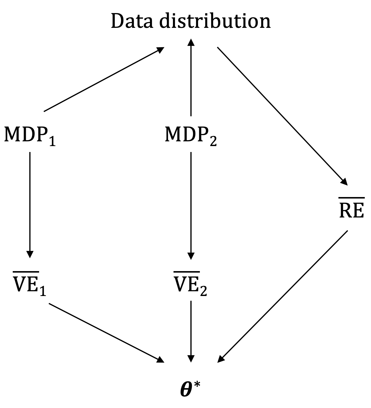 |
| Image from Reinforcement Learning: An Introduction (2018) by Richard S. Sutton and Andrew G. Barto. Because two different MDPs can produce the same data distribution but yield different mean squared value errors, \(\overline{\text{VE}}\) itself is not learnable. However, the parameter vector that minimizes \(\overline{\text{VE}}\) can be learned by minimizing \(\overline{\text{RE}}\). |
Bootstrapping Objectives
While value error and return error are appropriate criteria for approximate MC methods, these objectives are unsuitable for temporal difference (TD) methods due to their reliance on bootstrapping. Specifically, in MC methods, the update target is \(Y_t = G_t\). TD methods, by contrast, update \(\hat{V}(\theta)\) at each time step, before the final outcome \(G_t\) is known. Objectives based on the full return, such as the Return Error, are therefore not directly applicable to TD methods.
Value error is a problematic criterion for bootstrapping methods because the bootstrapped target is a biased estimate of \(V_\pi\). Specifically, in MC methods, the target \(Y_t = G_t\) provides an unbiased estimate of \(V_\pi\) since \(\mathbb{E}[G_t \mid s_t = s] = V_\pi(s) \; \forall t\). In bootstrapping methods, however, the update target is defined as \(Y_t = r_{t+1} + \gamma \hat{V}(s_{t+1}; \theta_t)\), which depends on the current parameter \(\theta_t\) and is therefore a “moving target.” When \(\theta\) is updated to reduce the error between \(Y_t\) and \(\hat{V}\), the target value \(Y_t\) itself changes. This dependence introduces bias into the estimate, making value error inappropriate for bootstrapping-based methods because convergence to a local optimum is guaranteed only when using an unbiased estimator. Thus, TD methods instead minimize Bellman-based objectives including Bellman error, projected Bellman error, and TD error.
Bellman Error
Bellman error can be derived from the state-value Bellman expectation equation:
\[ \begin{equation*} V_\pi(s) = \sum_{a \in \mathcal{A}} \pi(a \mid s) \left( R(s, a) + \gamma \sum_{s’ \in \mathcal{S}} P(s, a, s’) V_\pi(s’) \right) \;. \end{equation*} \]
As demonstrated in the DP for MDPs proofs note, the true value function is the unique fixed point of the Bellman operator, \(\mathcal{T}_\pi\). A fixed point of a transformation \(f\) is defined as a point \(p\) such that \(f(p) = p\). Intuitively, the true value function \(V_\pi\) is the only function that remains unchanged when the Bellman operator is applied. That is, applying \(\mathcal{T}_\pi\) to \(V_\pi\) yields \(V_\pi\) itself.
To quantify deviations from this fixed point, we define the Bellman error as the difference between the current estimate and its update under the Bellman operator. Mathematically, the Bellman error is given by:
\[ \begin{align} \overline{\delta}_{\theta}(s) &= [\mathcal{T}_\pi \hat{V}(\theta)](s) - \hat{V}(s; \theta) \label{eq:bellman-error-1} \\ &= \sum_{a \in \mathcal{A}} \pi(a \mid s) \left[ R(s, a) + \gamma \sum_{s’ \in \mathcal{S}} P(s, a, s’) \hat{V}(s’; \theta) \right] - \hat{V}(s; \theta) \label{eq:bellman-error-2} \\ &= \mathbb{E}_\pi \left[ r_{t+1} + \gamma \hat{V}(s_{t+1}; \theta) - \hat{V}(s_t; \theta) \mid s_t = s \right] \;. \label{eq:bellman-error-3} \end{align} \]
This formulation emphasizes that the Bellman error measures the inconsistency between an approximated value function \(\hat{V}(\theta)\) and its update under the Bellman operator, \(\mathcal{T}_\pi\). The error thus reflects how far \(\hat{V}(\theta)\) is from satisfying the Bellman equation.
As expressed in Equation \(\eqref{eq:bellman-error-2}\), the Bellman error includes an expectation over all possible next states \(s'\), weighted by the transition probabilities \(P(s, a, s’)\). However, because \(P(s, a, s’)\) is typically unknown in practice, the Bellman error cannot be computed exactly. Instead, it is estimated by sampling transitions from the environment, as demonstrated in Equation \(\eqref{eq:bellman-error-3}\). By accumulating multiple transitions from a given state \(s\) while following policy \(\pi\), we can calculate the average error over these samples. This yields an unbiased estimate of the Bellman error, allowing us to approximate it in the absence of full knowledge of the transition dynamics.
From Equations \(\eqref{eq:squared-norm-of-vector}\) and \(\eqref{eq:bellman-error-1}\), we can define the mean squared Bellman error as:
\[ \begin{equation*} \overline{\text{BE}} = \| \overline{\delta}_{\theta} \|_\mu^2 \;. \end{equation*} \]
TD Error vs. Bellman Error
The Bellman error is a theoretical construct closely related to the more practical temporal difference (TD) error. The TD error is a stochastic quantity computed from a single sampled transition \((s_t, a_t, r_{t+1}, s_{t+1})\), defined as
\[ \begin{equation*} \delta_t = r_{t+1} + \gamma \hat{V}(s_{t+1}; \theta) - \hat{V}(s_t; \theta) \;. \end{equation*} \]
Since the next state \(s_{t+1}\) and reward \(r_{t+1}\) are random variables, the TD error \(\delta_t\) is also random.
The Bellman error (Equation \(\eqref{eq:bellman-error-3}\)), is the expectation of the TD error at a given state \(s\). Formally:
\[ \begin{equation*} \overline{\delta}_{\theta}(s) = \mathbb{E}_\pi \left[ \delta_t \mid s_t = s \right] \;. \end{equation*} \]
This expectation is taken over the policy's action distribution and the environment's transition dynamics. Thus, the Bellman error at state \(s\) corresponds to the average TD error over all possible next states and rewards reachable from \(s\).
The relationship between TD error and Bellman error can be summarized as follows: The TD error is a stochastic, sample-based estimate of the Bellman error. It is computationally efficient, requiring only a single transition, but exhibits high variance. The Bellman error is the true expected error at a state. It is deterministic with zero variance. While it could, in principle, be approximated by generating many transitions from the same state \(s\) and averaging the resulting TD errors:
\[ \begin{equation*} \overline{\delta}_{\theta}(s) \approx \frac{1}{N} \sum_{i=1}^{N} \left[ r_{t+1}^{(i)} + \gamma \hat{V}(s_{t+1}^{(i)}; \theta) - \hat{V}(s; \theta) \right] \;, \end{equation*} \]
this approach is impractical in most RL settings as it would require repeatedly resetting the environment to state \(s\) to obtain a sufficient number of samples for each update.
Projected Bellman Error
By design, an approximate value function \(\hat{V}(\theta)\) cannot fully represent the complexity of the true value function \(V_\pi\). Specifically, the set of all possible value functions \(\mathcal{V}\) contains a subspace \(\hat{V}(\Theta)\), which comprises all the value functions representable by the chosen function approximator. For instance, if a linear function approximator is used, \(\hat{V}(\Theta)\) includes only linear functions. Because \(\hat{V}(\Theta)\) is typically much smaller than \(\mathcal{V}\), applying the Bellman operator to \(\hat{V}(\theta)\) is likely to produce a value function outside the representable subspace \(\hat{V}(\Theta)\). To address this, after each application of the Bellman operator, \(\hat{V}(\theta)\) can be projected back into the representable subspace using a projection operator \(\Pi\). Therefore, instead of minimizing the Bellman error directly, we can minimize the projected Bellman error:
\[ \begin{equation*} \overline{\text{PBE}}(\theta) = \| \Pi \overline{\delta}_{\theta} \|_\mu^2 \;, \end{equation*} \]
where \(\Pi\) is a projection operator that maps an arbitrary value function to the closest representable function. Formally, the projection is defined as:
\[ \begin{equation*} \Pi V = \hat{V}(\theta) \quad \text{where} \quad \theta = \arg\min_{\theta \in \mathbb{R}^d} \| V - \hat{V}(\theta) \|_\mu^2 \;. \end{equation*} \]
For a linear function approximator, there always exists an approximate value function for which the projected Bellman error (\(\overline{\text{PBE}}\)) equals zero. This solution is referred to as the TD fixed point. In general, this fixed point differs from the solutions obtained by methods that minimize value error (\(\overline{\text{VE}}\)) or Bellman error (\(\overline{\text{BE}}\)). However, as illustrated in the deadly triad note, the TD fixed point is not always stable when semi-gradient TD methods are used with off-policy training.
The Projection Operator with Linear Function Approximation
To illustrate the concept of projection, consider a linear function approximator, which expresses value estimates as a weighted sum of features:
\[ \begin{equation}\label{eq:values_to_estimate} \hat{V}(s; \theta) = \sum_{i=1}^d \theta_i \phi_i(s) = \theta^\top \phi(s) \;, \end{equation} \]
where \(\phi : \mathcal{S} \rightarrow \mathbb{R}^d\) maps states to \(d\)-dimensional feature vectors. Each component \(\phi_i(s)\) of vector \(\phi(s)\) is a feature of state \(s\), and each function \(\phi_i : \mathcal{S} \rightarrow \mathbb{R}\) is a basis function (so named because the features form a linear basis for the set of approximate functions).
Because the linear approximator is inherently less expressive than the true function, \(V_\pi\) is projected onto the subspace of representable (i.e., linear) functions using a projection operator. For a linear function approximator, this operator is also linear and can be represented as an \(|\mathcal{S}| \times |\mathcal{S}|\) matrix.
To formalize this projection, define \(\mathbf{v}_\pi \in \mathbb{R}^{|\mathcal{S}|} = [V_\pi(s_1), V_\pi(s_2), V_\pi(s_{|\mathcal{S}|})]^\top\) and \(\mathbf{D}\) as an \(|\mathcal{S}| \times |\mathcal{S}|\) diagonal matrix, with the state distribution \(\mu(s)\) along its diagonal. Let \(\Phi\) be an \(\mathcal |{S}| \times d\) matrix, wherein rows are the feature vectors \(\phi(s)^\top\), one for each state \(s\). The squared norm of a vector under the distribution \(\mu\) can then be expressed as:
\[ \begin{equation*} \| \mathbf{v} \|_\mu^2 = \mathbf{v}^\top \mathbf{D} \mathbf{v} \;. \end{equation*} \]
The objective is to determine the parameter vector \(\theta\) such that the projection \(\mathbf{v}_\theta = \Phi \theta\), which is the set of approximate values produced by Equation \(\eqref{eq:values_to_estimate}\) for all states, minimizes the \(\mu\)-weighted squared error with respect to \(\mathbf{v}_\pi\). More formally:
\[ \begin{align*} \min_{\theta} \| \mathbf{v}_\pi - \Phi \theta \|_\mu^2 &= \min_{\theta} (\mathbf{v}_\pi - \Phi \theta)^\top \mathbf{D} (\mathbf{v}_\pi - \Phi \theta) \\ &= \min_{\theta} \left( \mathbf{v}_\pi^\top \mathbf{D} \mathbf{v}_\pi - \mathbf{v}_\pi^\top \mathbf{D} \Phi \theta - (\Phi \theta)^\top \mathbf{D} \mathbf{v}_\pi + (\Phi \theta)^\top \mathbf{D} (\Phi \theta) \right) \\ &= \min_{\theta} \left( \mathbf{v}_\pi^\top \mathbf{D} \mathbf{v}_\pi - 2 \theta^\top \Phi^\top \mathbf{D} \mathbf{v}_\pi + \theta^\top \Phi^\top \mathbf{D} \Phi \theta \right). \end{align*} \]
To find the minimizing \(\theta\), we first take the derivative of the objective function with respect to \(\theta\):
\[ \begin{equation*} \nabla_\theta \left( \mathbf{v}_\pi^\top \mathbf{D} \mathbf{v}_\pi - 2 \theta^\top \Phi^\top \mathbf{D} \mathbf{v}_\pi + \theta^\top \Phi^\top \mathbf{D} \Phi \theta \right) = -2 \Phi^\top \mathbf{D} \mathbf{v}_\pi + 2 \Phi^\top \mathbf{D} \Phi \theta \;. \end{equation*} \]
Then we set the derivative equal to zero and solve for \(\theta\):
\[ \begin{align*} -2 \Phi^\top \mathbf{D} \mathbf{v}_\pi + 2 \Phi^\top \mathbf{D} \Phi \theta &= 0 \\ \Phi^\top \mathbf{D} \Phi \theta &= \Phi^\top \mathbf{D} \mathbf{v}_\pi \\ \theta &= \left( \Phi^\top \mathbf{D} \Phi \right)^{-1} \Phi^\top \mathbf{D} \mathbf{v}_\pi \;. \end{align*} \]
Thus, our projection is defined as:
\[ \begin{equation*} \Phi \theta = \Phi \left( \Phi^\top \mathbf{D} \Phi \right)^{-1} \Phi^\top \mathbf{D} \mathbf{v}_\pi \;. \end{equation*} \]
This entire expression can be interpreted as a linear operator that maps \(V_\pi\) onto the representable subspace. Thus, we define the projection operator \(\Pi\) as:
\[ \begin{equation*} \Pi = \Phi \left( \Phi^\top \mathbf{D} \Phi \right)^{-1} \Phi^\top \mathbf{D} \;. \end{equation*} \]
This definition of \(\Pi\) is derived from the concept of least-squares projection. Intuitively, \(\Pi \mathbf{v}_\pi\) provides the best approximation to \(\mathbf{v}_\pi\) within the subspace spanned by the feature vectors in \(\Phi\), measured under the distribution \(\mu\).
TD Error
The mean squared TD error is the average squared TD error, weighted by the frequency of state visits under a given policy. Mathematically, it is given by:
\[ \begin{align} \overline{\text{TDE}}(\theta) &= \sum_{s \in \mathcal{S}} \mu(s) \mathbb{E}[\delta_t^2 \mid s_t = s, a_t \sim \pi] \label{eq:sgd-td-loss-1} \\ &= \sum_{s \in \mathcal{S}} \mu(s) \mathbb{E}[\rho_t \delta_t^2 \mid s_t = s, a_t \sim \pi_\beta] \nonumber \\ &= \mathbb{E}_{\pi_\beta} [\rho_t \delta_t^2] \;, \label{eq:sgd-td-loss-2} \end{align} \]
where \(\mu\) is the distribution under \(\pi_\beta\), \(\delta_t = r_{t+1} + \gamma \hat{V}(s_{t+1}; \theta_t) - \hat{V}(s_t; \theta_t)\) is the one-step TD error with discounting, and \(\rho_t\) is the importance sampling ratio.
Equation \(\eqref{eq:sgd-td-loss-2}\) expresses the objective as an expectation over samples generated by the behavior policy \(\pi_\beta\). This representation allows unbiased gradient estimation from individual transitions, satisfying a fundamental requirement for stochastic gradient descent (SGD). Specifically, the expectation \(\mathbb{E}_{\pi_\beta}[\rho_t \delta_t^2]\) can be estimated using single transitions \((s, a, r, s’)\) collected under \(\pi_\beta\). For each transition, the TD error \(\delta_t\) and the importance sampling ratio \(\rho_t\) are computed. Their product, \(\rho_t \delta_t^2\), provides an unbiased estimate of the objective function. This unbiasedness follows directly from the definition of an unbiased estimator and is explicitly reflected in Equation \(\eqref{eq:sgd-td-loss-2}\). This contrasts with Equation \(\eqref{eq:sgd-td-loss-1}\), which requires enumerating the entire state space and sampling actions from the target policy \(\pi\) — operations typically infeasible in practice.
The Learnability of Bootstrapping Objectives
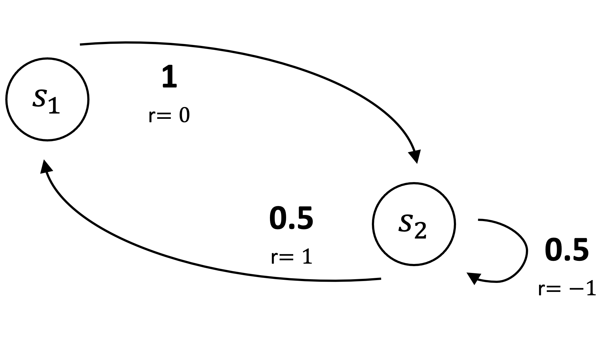
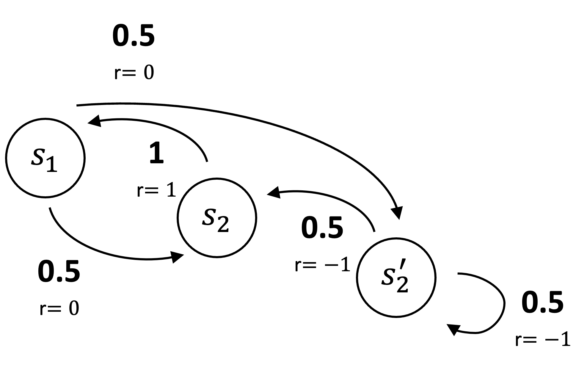
Like the value and return errors, the Bellman error is unlearnable. To illustrate, consider two additional MRPs. The first is a two-state system where the agent transitions deterministically from state \(s_1\) to \(s_2\), receiving a reward of \(0\). From state \(s_2\), the agent transitions to \(s_1\) with probability \(0.5\) and remains in \(s_2\) with probability \(0.5\), receiving rewards of \(1\) and \(-1\), respectively. States \(s_1\) and \(s_2\) have distinct representations \(\phi\).
 |
The second is a three-state MRP. In this system, the agent transitions from state \(s_1\) to \(s_2\) with probability \(0.5\) and to \(s_2'\) with probability \(0.5\), receiving a reward of \(0\) in both cases. From state \(s_2\), the agent always transitions back to \(s_1\), earning a reward of \(1\). From state \(s_2'\), the agent transitions to \(s_2\) with probability \(0.5\) and to \(s_2'\) with probability \(0.5\), with both transitions yielding a reward of \(-1\).
The states \(s_2\) and \(s_2'\) cannot be distinguished by their feature representations and are therefore assigned the same approximate value. Specifically, we use a two-component linear function approximator with feature vectors \(\phi(s_1) = [1,\,0]^\top\), \(\phi(s_2) = [0,\,1]^\top\), and \(\phi(s_2’) = [0,\,1]^\top\). With a parameter vector \(\theta = [\theta_1,\,\theta_2]^\top\), the approximate values are \(\hat{V}(s_1) = \theta_1\) and \(\hat{V}(s_2) = \hat{V}(s_2’) = \theta_2\).
For this example, we use a uniform weighting distribution \(\mu(s) = \tfrac{1}{3}\) over the three states.
 |
As in the \(\overline{\text{VE}}\) example, the observable data distribution is identical for the two MRPs. The agent observes \(s_1\) followed by a reward of \(0\), then a sequence of apparent \(s_2\)s. For both MRPs, the probability observing \(k\) apparent \(s_2\)s is \(2^{-k}\). Each observed \(s_2\) in the sequence is followed by a reward of \(-1\), except for the final \(s_2\), which is followed by a reward of \(1\). This process then repeats from \(s_1\).
First, we compute the Bellman Error \(\overline{\delta}_{\theta}(s) = \mathbb{E}[r’ + \gamma \hat{V}(s’;\theta)] - \hat{V}(s;\theta)\) for each state. With \(\gamma=0\) and \(\theta=0\) (so \(\hat{V}(s;\theta)=0\) for all \(s\)):
\[ \begin{align*} \overline{\delta}_{\theta}(s_1) &= \mathbb{E}[r’ \mid s_1] - \hat{V}(s_1;\theta) = 0 - 0 = 0 \\ \overline{\delta}_{\theta}(s_2) &= \mathbb{E}[r’ \mid s_2] - \hat{V}(s_2;\theta) = (0.5 \cdot 1 + 0.5 \cdot -1) - 0 = 0 \end{align*} \]
The Mean Squared Bellman Error is the weighted sum of these squared errors:
\[ \begin{equation*} \overline{\text{BE}}_1(\theta) = \frac{1}{2} (\overline{\delta}_{\theta}(s_1))^2 + \frac{1}{2} (\overline{\delta}_{\theta}(s_2))^2 = \frac{1}{2}(0)^2 + \frac{1}{2}(0)^2 = 0 \;. \end{equation*} \]
Similarly, for the second MRP, we first compute the Bellman Error for each state:
\[ \begin{align*} \overline{\delta}_{\theta}(s_1) &= \mathbb{E}[r’ \mid s_1] - \hat{V}(s_1;\theta) = 0 - 0 = 0 \\ \overline{\delta}_{\theta}(s_2) &= \mathbb{E}[r’ \mid s_2] - \hat{V}(s_2;\theta) = 1 - 0 = 1 \\ \overline{\delta}_{\theta}(s_2’) &= \mathbb{E}[r’ \mid s_2'] - \hat{V}(s_2’;\theta) = -1 - 0 = -1 \end{align*} \]
The Mean Squared Bellman Error is then:
\[ \begin{equation*} \overline{\text{BE}}_2(\theta) = \frac{1}{3}(\overline{\delta}_{\theta}(s_1))^2 + \frac{1}{3}(\overline{\delta}_{\theta}(s_2))^2 + \frac{1}{3}(\overline{\delta}_{\theta}(s_2’))^2 = \frac{1}{3}(0)^2 + \frac{1}{3}(1)^2 + \frac{1}{3}(-1)^2 = \frac{2}{3} \;. \end{equation*} \]
As with the value error, the Bellman error differs between two MRPs that produce identical data distributions demonstrating that the Bellman error is not learnable. Unlike \(\overline{\text{VE}}\), however, it is not possible to learn the parameter for which \(\overline{\text{BE}}\) is optimal. In the first MRP, \(\theta = 0\) is optimal regardless of the value of \(\gamma\). In the second MRP, the optimal \(\theta\) is a complex function of \(\gamma\), but as \(\gamma \to 1\), the optimal value approaches \((-1/3, 1/6)^\top\).
The other bootstrapping objectives, \(\overline{\text{PBE}}\) and \(\overline{\text{TDE}}\), are learnable from the available data. The figure below summarizes the learnability of the three bootstrapping objectives described in this note.
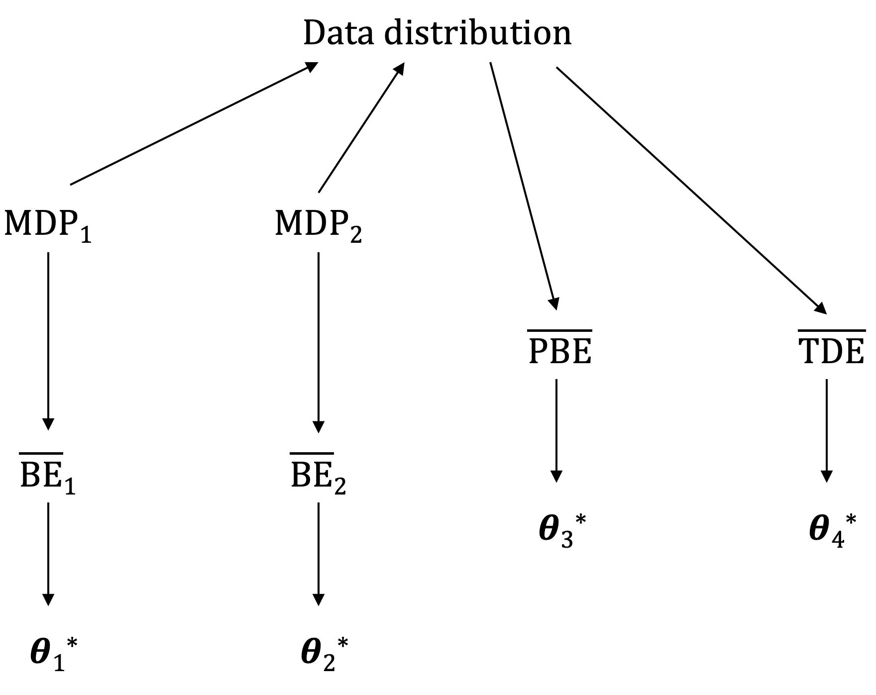 |
| Image from Reinforcement Learning: An Introduction (2018) by Richard S. Sutton and Andrew G. Barto. Two distinct Markov decision processes (MDPs) can generate identical data distributions but have different Bellman errors and minimizing parameter vectors. Consequently, Bellman error values cannot be learned, even with infinite data. Both the projected Bellman error and the TD error, along with their respective minima, can be directly learned from data. However, the parameter vectors minimizing these two objectives will generally differ. |
Citation
Landers, Matthew. "The Learnability of RL Objectives." mattlanders.net, December 12, 2024. mattlanders.net/learnability-of-rl-objectives.
@article{landers2024learnability,
  title = {The Learnability of RL Objectives},
  author = {Landers, Matthew},
  journal = {mattlanders.net},
  year = {2024},
  month = {December},
  url = "mattlanders.net/learnability-of-rl-objectives"
}
References
- Reinforcement Learning: An Introduction (2018)
Richard S. Sutton and Andrew G. Barto
- TD error vs advantage vs Bellman error (2017)
Boris Belousov