Implicit Q-Learning
Revised September 28, 2025
The Deep Q-Learning note is optional but recommended background reading.
Offline reinforcement learning assumes access to a fixed dataset \(\mathcal{B} = \{(s_t,a_t,r_t,s_{t+1})\}_{t=1}^Z\) generated by a behavior policy \(\pi_b\), which may be optimal, suboptimal, or a mixture of policies. The learning agent has no additional access to the environment and must train entirely from this static dataset. In offline RL the maximization in the mean squared Bellman error:
\[ \begin{equation*} L_{TD}(\theta) = \mathbb{E}_{(s,a,r,s’) \sim \mathcal{B}} \left[ \left(r + \gamma \max_{a’} Q(s’, a’) - Q(s, a) \right)^2 \right] \;, \end{equation*} \]
induces systematic overestimation. For actions \(a'\) outside the support of \(\mathcal{B}\) the estimates \(Q(s’,a’;\hat{\theta})\) are purely extrapolated, since \(\mathcal{B}\) provides no evidence for their value. If such actions receive spuriously high estimates the \(\max\) operator selects them and Bellman updates propagate the bias through successive targets. In online RL such errors can be corrected by evaluating actions through additional environmental interaction. Offline RL lacks this validation, so extrapolated estimates persist. Reliable offline learning therefore requires constraining policies to the support of \(\mathcal{B}\). Common approaches penalize out-of-distribution actions through value regularization or constrain the learned policy directly, though these methods do not fully prevent extrapolation error.
Implicit Q-Learning (IQL) mitigates extrapolation error by (i) learning a state-value \(V(s)\) via expectile regression over in-dataset action values \(Q(s,a)\), and then (ii) training \(Q\) with targets \(r+\gamma V(s’)\). This replaces the explicit maximization over (potentially out-of-support) actions and biases value estimates toward higher in-support actions through the expectile parameter \(\tau\).
Expectile Regression
Out-of-distribution actions can be trivially avoided by defining the backup only with actions \(a'\) sampled from the dataset:
\[ \begin{equation}\label{eq:sarsa-like-loss} L(\theta) = \mathbb{E}_{(s,a,r,s’,\color{red}{a’})\sim\mathcal{B}} \left[\big(r + \gamma Q(s’,a’;\hat{\theta}) - Q(s,a;\theta)\big)^2\right], \end{equation} \]
Equation \(\eqref{eq:sarsa-like-loss}\) recovers the Q-function of the behavior policy, \(Q^{\pi_b}\). A new policy \(\pi\) can then be extracted by \(\arg \max_a Q^{\pi_b}(s,a)\), which corresponds to a single step of policy iteration — first evaluate the behavior policy, then take the greedy improvement. Such one-step dynamic programming methods, however, are known to fail on complex tasks.
The loss in Equation \(\eqref{eq:sarsa-like-loss}\) minimizes the Bellman error under the behavior policy, yielding the average action value under \(\pi_b\):
\[ \begin{equation*} \mathbb{E}_{a \sim \pi_b}[Q(s,a)] \;. \end{equation*} \]
The mean arises because squared error penalizes positive and negative deviations symmetrically. To bias the estimate toward higher values supported by the dataset, IQL replaces MSE with expectile regression. For a distribution \(X\), the \(\tau\)-expectile \(m_\tau\) is defined by:
\[ \begin{equation}\label{eq:expectile} m_\tau = \arg\min_m \mathbb{E}_{x \sim X}\big[L_2^\tau(x-m)\big] \;, \end{equation} \]
with asymmetric loss:
\[ \begin{equation*} L_2^\tau(u) = |\tau - \mathbf{1}_{\{u<0\}}| u^2 \;. \end{equation*} \]
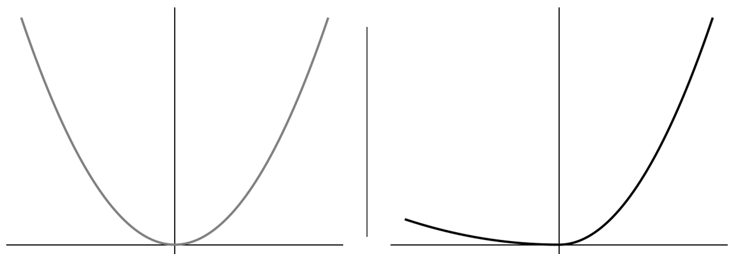 |
| The mean-squared loss (left) penalizes positive and negative errors symmetrically, with weight growing quadratically in the error magnitude. The expectile loss (right) introduces asymmetry: for \(\tau>0.5\) (here \(\tau=0.9\)), positive errors \(r + \gamma Q(s’,a’;\hat{\theta}) - Q(s,a;\theta) > 0\) are penalized more heavily than negative errors. Underestimates of the target therefore incur larger loss than overestimates, biasing the solution upward toward the upper tail of the distribution. |
An expectile can be viewed as a squared analogue of a quantile. The first-order condition of Equation \(\eqref{eq:expectile}\) is:
\[ \begin{equation*} \mathbb{E}\big[(\tau-\mathbf{1}_{\{X<m_\tau\}})(X-m_\tau)\big] = 0 \;. \end{equation*} \]
When \(\tau\) increases, positive deviations \((X-m_\tau)>0\) are weighted more heavily, so \(m_\tau\) shifts upward. As \(\tau \to 1\), the weight on negative deviations vanishes and \(m_\tau\) approaches the supremum of the support of \(X\). Applied to the distribution of \(Q(s,a)\) under \(a \sim \pi_b(\cdot\mid s)\), the \(\tau\)-expectile interpolates between the mean action value (\(\tau=0.5\)) and, in the limit, the maximum in-support action value:
\[ \begin{equation*} \lim_{\tau \to 1} \text{Expectile}_\tau\big(Q(s,a), a \sim \pi_b(\cdot\mid s)\big) = \max_{a \in \Omega(s)} Q(s,a) \;, \end{equation*} \]
where \(\Omega(s)=\{a \in A : \pi_b(a\mid s) > 0\}\) denotes the dataset support.
Thus when used as the target in the SARSA-style update (Equation \(\eqref{eq:sarsa-like-loss}\)), the expectile value function trains the Q-function to approximate the maximum value attainable from actions in the support of \(\pi_b\):
\[ \begin{equation*} L_{TD}(\theta) = \mathbb{E}_{(s,a,r,s’) \sim \mathcal{B}} \Big[ \big(r + \gamma \max_{a’ \in \Omega(s)} Q(s’,a’;\hat{\theta}) - Q(s,a;\theta)\big)^2 \Big] \;. \end{equation*} \]
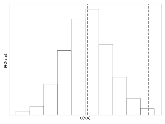 |
| If \(Q\) generalizes, each state \(s \in \mathcal{B}\) induces a distribution of action values \(Q(s,a)\) under \(\pi_b\), shown by the histogram. Minimizing mean-squared error yields the expectation of this distribution (gray line), corresponding to the average action value. Expectile regression instead shifts the estimate upward: for \(\tau>0.5\), positive deviations receive larger weight than negative deviations, so the estimate (black line) lies above the mean. |
A naive approach to bias Q-learning toward higher in-support values would be to replace the squared loss in Equation \(\eqref{eq:sarsa-like-loss}\) with an asymmetric expectile loss:
\[ \begin{equation}\label{eq:expectile-loss} L(\theta) = \mathbb{E}_{(s,a,r,s’,a’) \sim \mathcal{B}} \left[ L_2^\tau \left(r + \gamma Q(s’,a’;\hat{\theta}) - Q(s,a;\theta)\right) \right] \;, \end{equation} \]
For \(\tau > 0.5\), positive errors \(u>0\) receive larger weight than negative errors \(u<0\). That is, underestimates of the target are penalized more heavily than overestimates. The resulting estimator is biased upward, shifting \(Q(s,a;\theta)\) toward the upper tail of the distribution of returns.
However, applying expectile regression directly to the Bellman targets conflates two sources of variability: the action distribution under \(\pi_b\) and stochasticity in the transition dynamics \(s’ \sim P(\cdot \mid s,a)\). A “lucky” high target can arise from rare transitions rather than systematically good actions. IQL therefore does not use expectile loss for \(Q\). Instead, it applies expectile regression only to learn a state-value \(V(s)\) over in-dataset actions, and then trains \(Q\) with standard mean-squared error toward the target \(r + \gamma V(s’)\).
The loss in Equation \(\eqref{eq:expectile-loss}\) mitigates overestimation but does not isolate the contribution of the action distribution — its targets also reflect stochasticity from the dynamics \(s’ \sim P(\cdot \mid s,a)\). A “lucky”, high value of \(r + \gamma Q(s’,a’;\hat{\theta})\) may therefore arise from a rare positive transition rather than the typical value of an action. Thus, IQL trains a separate value function \(V_\psi\) that estimates an expectile with respect only to the action distribution:
\[ \begin{equation*} L_V(\psi) = \mathbb{E}_{(s,a) \sim \mathcal{B}} \Big[ L_2^\tau \big(Q(s,a;\hat{\theta}) - V(s;\psi)\big) \Big] \;. \end{equation*} \]
The expectile value \(V_\psi\) then defines the targets for Q-learning through a mean-squared loss:
\[ \begin{equation}\label{eq:iql-loss} L_Q(\theta) = \mathbb{E}_{(s,a,r,s’) \sim \mathcal{B}} \Big[\big(r + \gamma V(s’;\psi) - Q(s,a;\theta)\big)^2\Big] \;. \end{equation} \]
Using \(V_\psi\) averages over transition stochasticity, avoiding spurious targets from rare “lucky” outcomes.
Recovering a Policy
Equation \(\eqref{eq:iql-loss}\) trains \(Q\) toward targets \(r+\gamma V(s’)\), where \(V\) is an upper-biased in-support estimate (controlled by \(\tau\)). This implicitly favors higher in-support actions without taking an explicit \(\max\). The policy for which these Q-values are approximated is “implicit” — the Bellman update evaluates the policy that selects the maximal in-support action, but this policy is never constructed explicitly. Greedy extraction from \(Q\) is unstable in the offline setting, since \(\max_{a’} Q(s,a’)\) may still favor unsupported actions. IQL therefore extracts the policy with a constrained method, advantage-weighted regression (AWR).
AWR fits a parametric policy \(\pi_\phi\) to the dataset actions while reweighting them according to their advantage:
\[ \begin{equation*} A(s,a) = Q(s,a) - V(s) \;, \end{equation*} \]
so that actions with higher advantage are imitated more strongly. Concretely, the policy is obtained by minimizing the weighted log-loss
\[ \begin{equation*} L_\pi(\phi) = \mathbb{E}_{(s,a)\sim \mathcal{B}} \left[ - \exp\!\left(\tfrac{A(s,a)}{\beta}\right)\,\log \pi_\phi(a\mid s) \right] \;, \end{equation*} \]
where \(\beta>0\) is a temperature parameter controlling how aggressively the policy concentrates on high-advantage actions. This procedure ensures that policy learning remains within the dataset support, while still biasing toward actions that improve on \(\pi_b\).
 |
Citation
Landers, Matthew. "Implicit Q-Learning." mattlanders.net, September 28, 2025. mattlanders.net/implicit-q-learning.
@article{landers2025implicit,
  title = {Implicit Q-Learning},
  author = {Landers, Matthew},
  journal = {mattlanders.net},
  year = {2025},
  month = {September},
  url = "mattlanders.net/implicit-q-learning"
}
References
- Offline Reinforcement Learning with Implicit Q-Learning (2021)
Ilya Kostrikov, Ashvin Nair, and Sergey Levine
- CS 285 at UC Berkeley: Deep Reinforcement Learning. Lecture 15, Part 1: Offline Reinforcement Learning [video] (2021)
Sergey Levine
- CS 285 at UC Berkeley: Deep Reinforcement Learning. Lecture 16, Part 1: Offline Reinforcement Learning 2 [video] (2021)
Sergey Levine
- Implicit Q Learning (2023)
Robert Müller
- Advantage-Weighted Regression: Simple and Scalable Off-Policy Reinforcement Learning (2019)
Xue Bin Peng, Aviral Kumar, Grace Zhang, and Sergey Levine