Bayes’ Theorem for Probability Distributions
Revised July 10, 2025
Bayesian statistics provides a principled approach for incorporating prior knowledge into statistical inference. In this framework, uncertainty about an unknown parameter is encoded using a probability distribution, known as the prior. As data are observed, this prior is updated to a posterior distribution, which reflects both the prior belief and the evidence provided by the data. With increasing sample size, the posterior typically becomes less sensitive to the prior, allowing the data to dominate the inference.
Consider estimating the proportion of women in a university population. Let \(X_1, \dots, X_n\) be independent binary observations drawn with replacement, where \(X_i = 1\) indicates a woman and \(X_i = 0\) otherwise. A standard point estimate of the proportion \(\theta \in [0,1]\) is the empirical mean:
\[ \begin{equation*} \hat{\theta} = \frac{1}{n} \sum_{i=1}^n X_i \;, \end{equation*} \]
which coincides with the maximum likelihood estimate under a Bernoulli model. While this estimate is efficient in large samples, it can behave poorly when \(n\) is small — for example, producing \(\hat{\theta} = 0\) or \(1\), which are extreme and implausible. Bayesian estimators incorporate prior information and naturally regularize such estimates toward more reasonable values, such as \(\theta \approx 0.5\).
In the Bayesian framework, \(\theta\) is treated as a random variable. Uncertainty about its value is encoded by a probability distribution over \([0,1]\), reflecting subjective belief rather than inherent randomness. This contrasts with the frequentist approach, which regards \(\theta\) as a fixed but unknown constant and does not assign it a probability distribution.
Bayesian inference specifies a prior and a likelihood, which together determine the posterior distribution over \(\theta\). More specifically, the prior captures the initial belief about \(\theta\), and the likelihood models the data generation process conditional on \(\theta\). The posterior represents the distribution of \(\theta\) conditional on the observed data. It is obtained by combining the prior \(\pi(\theta)\) with the likelihood function \(p(\mathbf{X} \mid \theta)\) using Bayes’ theorem. This yields an updated distribution that reflects both prior belief and the evidence provided by the data. Repeated applications of this framework support sequential inference: the posterior after observing one dataset serves as the prior before observing the next.
Specifying the Prior Distribution
Returning to the university gender distribution example, consider the problem of specifying a prior distribution for the unknown parameter \(\theta \in [0,1]\), representing the proportion of women in the population. Prior uncertainty about \(\theta\) may be expressed through subjective probability statements — for example, assigning 90% probability to the interval \([0.4, 0.6]\) and 95% to \([0.3, 0.8]\). There are many ways to represent such beliefs, but not all choices are mathematically convenient. For instance, one could construct a custom multimodal distribution with several shape parameters, but this would complicate both analytical derivations and numerical computations.
Not all belief distributions are valid priors, as the model's parameter space constrains admissible choices. In particular, the prior's support must match the domain of the parameter. For Bernoulli-distributed observations, as in our example, this domain is \([0,1]\), making the Beta distribution a natural choice. The Beta family is defined over \([0,1]\) and parameterized by two positive shape parameters, \(\alpha\) and \(\beta\). It can express a wide variety of belief profiles — from uniform ignorance to sharply peaked certainty — while remaining analytically tractable. This flexibility enables the prior to capture both the location of belief (e.g., \(\theta \approx 0.5\)) and the strength of that belief. For example, a sharply peaked Beta distribution centered at \(0.5\) indicates a high degree of certainty in a roughly equal gender split, whereas a flatter distribution reflects greater uncertainty.
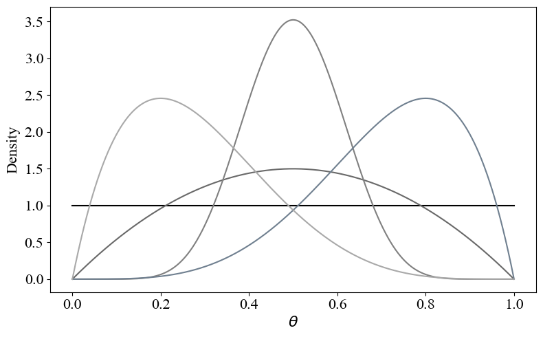 |
| Examples of Beta priors over \(\theta \in [0,1]\). The shape parameters \((\alpha, \beta)\) control both the location and concentration of belief, yielding uniform, symmetric, or skewed distributions. |
Although \(\theta\) itself is a fixed but unknown quantity, Bayesian analysis represents uncertainty about its value by modeling it as a random variable. The prior distribution \(\theta \sim \text{Beta}(\alpha, \beta)\) encodes this uncertainty. The use of probability to quantify epistemic uncertainty (rather than aleatoric randomness) is a defining feature of the Bayesian framework. Although the true value of \(\theta\) is not random in any physical sense, treating it as such for inference purposes provides a coherent and flexible modeling approach.
Generating the Data Based on the Parameters
Continuing with the university example, suppose the unknown parameter \(\theta\) represents the proportion of women in the population (about which we have a prior belief). Data are generated by sampling \(n\) individuals at random. Let \(X_i = 1\) if the \(i\)-th individual is a woman and \(X_i = 0\) otherwise. Assuming independent sampling (e.g., with replacement), the result is a sequence of conditionally independent Bernoulli trials, each with success probability \(\theta\).
Formally, the observations \(X_1, \dots, X_n\) are modeled as conditionally independent given \(\theta\):
\[ \begin{equation}\label{eq:data-generation} X_i \mid \theta \sim \text{Ber}(\theta) \;. \end{equation} \]
This sampling process is equivalent to flipping \(n\) independent biased coins. For example, if \(\theta = 0.75\), each \(X_i\) can be generated by drawing an independent value \(x_i \sim \text{Uniform}(0,1)\) and setting \(X_i = 1\) if \(x_i < \theta\), and \(X_i = 0\) otherwise.
Updating the Prior Belief
After observing data, the prior distribution over \(\theta\) is updated by conditioning on the observed sample using Bayes’ Theorem:
\[ \begin{equation*} P(A \mid B) = \frac{P(A \cap B)}{P(B)} = \frac{P(B \mid A)\, P(A)}{P(B)} \;, \end{equation*} \]
where \(P(A \mid B)\) corresponds to the posterior, \(P(B \mid A)\) to the likelihood, and \(P(A)\) to the prior. The continuous analogue is defined as:
\[ \begin{equation}\label{eq:posterior} \pi(\theta \mid \mathbf{X}) = \frac{p_n(\mathbf{X} \mid \theta) \pi(\theta)}{\int_\Theta p_n(\mathbf{X} \mid \theta) \pi(\theta) \, d\theta} \;. \end{equation} \]
where \(\pi(\cdot)\) is the prior density over the parameter space \(\Theta\), \(\mathbf{X} = (X_1, \dots, X_n)\) is the observed data, \(p_n(\cdot \mid \theta)\) is the joint probability mass function of \(\mathbf{X}\) given \(\theta\), and \(\pi(\theta \mid \mathbf{X})\) is the posterior density.
The denominator ensures normalization and is referred to as the marginal likelihood. In practice, it is often treated as a constant when focusing on the shape of the posterior. Evaluating Equation \(\eqref{eq:posterior}\) therefore reduces to computing the likelihood and the prior.
The prior \(\pi(\theta)\) is typically specified directly. The likelihood \(p_n(\mathbf{X} \mid \theta)\), by contrast, must be derived from the assumed data-generating process. It quantifies how probable the observed data are for each possible value of the parameter and serves as the conduit through which data influence the posterior.
Assume that conditioned on \(\theta \in [0,1]\), the data are independently distributed (Equation \(\eqref{eq:data-generation}\)). The Bernoulli distribution assigns probability \(\theta\) to \(X_i = 1\) and \(1 - \theta\) to \(X_i = 0\). For a given observation \(x_i \in \{0,1\}\), the mass function is:
\[ \begin{equation*} P(X_i = x_i \mid \theta) = \theta^{x_i}(1 - \theta)^{1 - x_i} \;. \end{equation*} \]
Conditional independence implies the likelihood factorizes:
\[ \begin{align} p_n(\mathbf{X} \mid \theta) &= \prod_{i=1}^n \theta^{X_i}(1 - \theta)^{1 - X_i} \nonumber \\ &= \theta^{\sum_{i=1}^n X_i}(1 - \theta)^{n - \sum_{i=1}^n X_i} && \text{collecting exponents} \nonumber \\ &= \theta^S(1 - \theta)^{n - S} \;, \label{eq:likelihood} \end{align} \]
where \(S = \sum_{i=1}^n X_i\) is the number of observed successes.
Assume the prior is Beta distributed: \(\theta \sim \text{Beta}(\alpha, \beta)\), with density proportional to:
\[ \begin{equation}\label{eq:beta-kernel} \pi(\theta) \propto \theta^{\alpha - 1}(1 - \theta)^{\beta - 1} \;. \end{equation} \]
Multiplying the likelihood and prior yields the unnormalized posterior:
\[ \begin{equation}\label{eq:unnormalized-posterior} \pi(\theta \mid \mathbf{X}) \propto \theta^S(1 - \theta)^{n - S} \cdot \theta^{\alpha - 1}(1 - \theta)^{\beta - 1} = \theta^{\alpha - 1 + S}(1 - \theta)^{\beta - 1 + n - S} \;. \end{equation} \]
Conjugate Prior
Multiplying the likelihood (Equation \(\eqref{eq:likelihood}\)) by the prior (Equation \(\eqref{eq:beta-kernel}\)) yields the unnormalized posterior in Equation \(\eqref{eq:unnormalized-posterior}\). This expression matches the kernel of a Beta distribution with updated parameters, allowing the posterior to be defined as:
\[ \begin{equation}\label{eq:posterior-beta} \theta \mid \mathbf{X} \sim \text{Beta}(\alpha + S, \; \beta + n - S) \;. \end{equation} \]
This example illustrates conjugacy. In general, a prior is conjugate to a likelihood if the resulting posterior distribution belongs to the same parametric family as the prior.
Conjugacy offers analytical convenience, as the posterior distribution belongs to the same parametric family as the prior. This allows the denominator in Equation \(\eqref{eq:posterior}\) to be obtained without evaluating the integral — it can simply be looked up. For example, for any Beta distribution with parameters \((a, b)\), the normalizing constant is the reciprocal of the Beta function \(B(a,b)\):
\[ \begin{equation*} \frac{1}{B(a,b)} = \frac{\Gamma(a + b)}{\Gamma(a)\, \Gamma(b)} \;, \end{equation*} \]
where \(\Gamma\) is the Gamma function. For a posterior \(\text{Beta}(\alpha_{post}, \beta_{post})\), the normalizing constant is computed by substituting \(a = \alpha_{post}\) and \(b = \beta_{post}\).
Non-conjugate priors, by contrast, typically yield posterior distributions without closed-form expressions, requiring numerical approximation of the normalizing constant.
Inference from the Posterior
Given observed data \(\mathbf{X} = (X_1, \dots, X_n)\) and a Beta prior \(\text{Beta}(\alpha, \beta)\), the posterior distribution over the unknown proportion \(\theta\) is \(\text{Beta}(\alpha_{post}, \beta_{post})\), where, by Equation \(\eqref{eq:posterior-beta}\):
\[ \begin{equation*} \alpha_{post} = \alpha + \sum_{i=1}^n X_i \;, \quad \beta_{post} = \beta + n - \sum_{i=1}^n X_i \;. \end{equation*} \]
This posterior encodes all available information about \(\theta\), combining prior beliefs and empirical observations under the specified model. Inference proceeds by computing relevant functionals of this distribution.
Point Estimates
Several scalar summaries of the posterior distribution \(\text{Beta}(\alpha_{post}, \beta_{post})\) serve as point estimates of \(\theta\), each minimizing a different loss function.
The posterior mean, which minimizes expected squared error loss, is given by
\[ \begin{equation*} \hat{\theta}_{\text{mean}} = \mathbb{E}[\theta \mid \mathbf{X}] = \frac{\alpha_{post}}{\alpha_{post} + \beta_{post}} = \frac{\alpha + \sum X_i}{\alpha + \beta + n} \;. \end{equation*} \]
This follows from the known expectation of the Beta\((\alpha, \beta)\) distribution. Such an estimate combines prior pseudo-counts \((\alpha, \beta)\) with empirical counts \((\sum X_i, n - \sum X_i)\), and converges to the empirical mean \(\hat{\theta} = \frac{1}{n} \sum X_i\) as \(n\) increases.
The posterior median minimizes expected absolute error and satisfies \(P(\theta \le m \mid \mathbf{X}) = 0.5\). While the Beta distribution has no closed-form expression for its median, it can be computed numerically via the inverse cumulative distribution function.
The posterior mode, or maximum a posteriori (MAP) estimate, maximizes the posterior density. For \(\alpha_{post} > 1\) and \(\beta_{post} > 1\), it is given by:
\[ \begin{equation*} \hat{\theta}_{\text{MAP}} = \frac{\alpha_{post} - 1}{\alpha_{post} + \beta_{post} - 2} = \frac{(\alpha - 1) + \sum X_i}{(\alpha - 1) + (\beta - 1) + n} \;. \end{equation*} \]
If \(\alpha_{post} \le 1\) or \(\beta_{post} \le 1\), the mode lies at the boundary or the distribution may be U-shaped. The MAP estimate generalizes the maximum likelihood estimate by incorporating prior regularization.
Credible Intervals
Bayesian inference permits interval estimates of \(\theta\) by identifying a region in which the posterior probability mass is concentrated. A \((1 - \gamma) \times 100\%\) credible interval is any interval \([L, U] \subset [0,1]\) such that:
\[ \begin{equation*} P(L \le \theta \le U \mid \mathbf{X}) = \int_L^U \pi(\theta \mid \mathbf{X})\, d\theta = 1 - \gamma \;. \end{equation*} \]
In the Bayesian framework, this quantity represents the probability that \(\theta\) lies within \([L, U]\), conditional on the observed data. In contrast to frequentist confidence intervals, which concern long-run coverage under repeated sampling, credible intervals characterize uncertainty about a fixed but unknown parameter.
Two constructions are standard and commonly used. The equal-tailed interval is defined by the \(\gamma/2\) and \(1 - \gamma/2\) quantiles of the posterior distribution. For a Beta posterior \(\text{Beta}(\alpha_{post}, \beta_{post})\), the bounds are given by:
\[ \begin{equation*} L = F^{-1}_{\text{Beta}}(\gamma/2; \alpha_{post}, \beta_{post}) \;, \quad U = F^{-1}_{\text{Beta}}(1 - \gamma/2; \alpha_{post}, \beta_{post}) \;, \end{equation*} \]
where \(F^{-1}_{\text{Beta}}\) denotes the inverse cumulative distribution function of the Beta distribution.
An alternative is the highest posterior density (HPD) interval, which contains the smallest-length interval \([L, U]\) such that:
\[ \begin{equation*} \int_L^U \pi(\theta \mid \mathbf{X})\, d\theta = 1 - \gamma \;, \end{equation*} \]
and every point inside the interval has posterior density at least as great as any point outside.
In many common cases, such as when the posterior is unimodal and the interval lies strictly within the support, the endpoints satisfy \(\pi(L \mid \mathbf{X}) = \pi(U \mid \mathbf{X})\). However, this condition does not hold in general. For example, when the posterior is U-shaped (e.g., \(\alpha_{\text{post}} < 1\) and \(\beta_{\text{post}} < 1\)), or when it concentrates at the boundary (e.g., \(\text{Beta}(0.5, 2)\)), the HPD interval may include \(0\) or \(1\) as an endpoint, where the density may be infinite or behave asymmetrically. In such cases, the defining property of the HPD interval is not that the density is equal at the endpoints, but that the interval is the shortest one containing the desired posterior mass.
Citation
Landers, Matthew. "Bayes' Theorem for Probability Distributions." mattlanders.net, July 10, 2025. mattlanders.net/bayes-theorem-for-probability-distributions.
@article{landers2025bayes,
  title = {Bayes' Theorem for Probability Distributions},
  author = {Landers, Matthew},
  journal = {mattlanders.net},
  year = {2025},
  month = {July},
  url = "mattlanders.net/bayes-theorem-for-probability-distributions"
}
References
- Basics of Bayesian Statistics, Introduction to Applied Bayesian Statistics and Estimation for Social Scientists (2007)
Scott M. Lynch
- Bayesian analysis, Stanford STATS 200: Introduction to Statistical Inference (2016)
Zhou Fan
- Bayesian Statistics [video], MIT 18.650 Statistics for Applications (2016)
Philippe Rigollet
- Bayesian Statistics (cont.) [video], MIT 18.650 Statistics for Applications (2016)
Philippe Rigollet
- Chapter 2: Bayes’ Theorem for Distributions Lecture Notes, Newcastle University MAS2317/3317: Introduction to Bayesian Statistics (2013)
Lee Fawcett