Proximal Policy Optimization (PPO)
Revised May 30, 2025
The TRPO note is optional but recommended background reading.
A code implementation of the method described in this note is available as optional supplementary material.
On-policy policy gradient methods are generally sample-inefficient as they compute a single policy update per trajectory, using returns that span the entire episode. Multiple updates per trajectory ostensibly improve efficiency, however this produces biased gradient estimates. Consider a trajectory \(\tau = \{(s_0, a_0, r_1), \dots, (s_T, a_T, r_{T+1})\}\) generated by the policy \(\pi_{\theta_\text{old}}\). Suppose the first segment of this trajectory — comprising tuples \((s_k, a_k, G_k)\) for time steps \(k = 0, \dots, m-1\) — is used to perform a policy update using the REINFORCE rule:
\[ \begin{equation*} \theta = \theta_\text{old} + \alpha \gamma^k G_k \nabla_\theta \ln \pi(a_k \mid s_k; \theta_\text{old}) \;, \end{equation*} \]
yielding a new policy \(\pi_\theta\). If a subsequent update is performed using data from a later segment of the same trajectory — for example, tuples \((s_j, a_j, G_j)\) for \(j = m, \dots, 2m-1\) — the update is no longer on-policy. That is, although the gradient is computed with respect to the updated policy \(\pi_{\theta}\), the data \((s_j, a_j, G_j)\) were generated under the previous policy \(\pi_{\theta_\text{old}}\). This violates the on-policy requirement that data used to estimate the policy gradient must be drawn from the current policy, thereby introducing bias into the gradient estimate and potentially leading to instability or divergence during training.
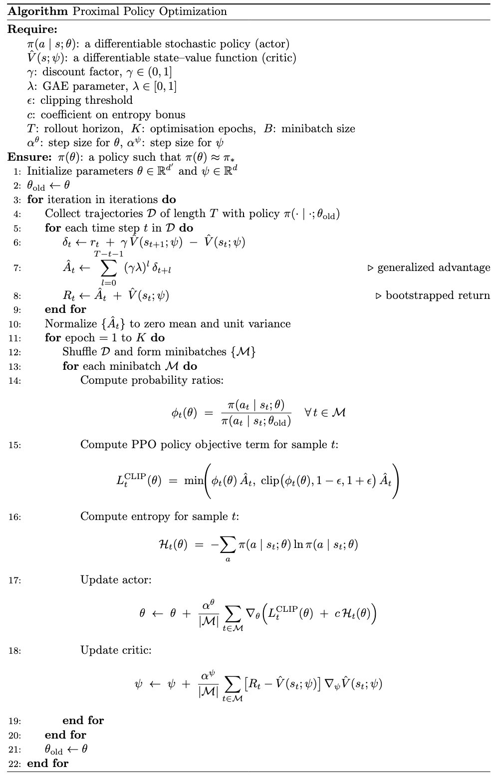
Proximal Policy Optimization (PPO) improves the sample efficiency of both vanilla policy gradient methods and TRPO by enabling multiple gradient updates on data from a single policy. To promote stable learning, it constrains the divergence between the updated policy \(\pi_\theta\) and the data-generating policy \(\pi_{\theta_\text{old}}\) using a clipped probability ratio. This surrogate objective limits how far the policy can shift during optimization, allowing repeated updates while maintaining approximate on-policy behavior.
PPO's learning objective is derived from TRPO's theoretically grounded policy iteration framework:
\[ \begin{equation}\label{eq:trpo-max-problem} \max_\theta \mathbb{E}_{(s_t, a_t) \sim \pi_{\theta_\text{old}}} \left[ \color{red}{\frac{\pi(a_t \mid s_t; \theta)}{\pi(a_t \mid s_t; \theta_\text{old})} A(s_t, a_t; \theta_\text{old})} - \color{blue}{C \max_s D_{KL} \left( \pi_{\theta_\text{old}}(\cdot \mid s) \,\|\, \pi_\theta(\cdot \mid s) \right)} \right] \;. \end{equation} \]
Equation \(\eqref{eq:trpo-max-problem}\) guarantees monotonic policy improvement by penalizing large deviations from the reference policy via the KL-divergence term (highlighted in blue). In practice, however, tuning the penalty coefficient \(C\) is challenging and often leads to overly conservative updates. Moreover, the expectation assumes exact computation over the state-action distribution induced by \(\pi_{\theta_\text{old}}\), which is typically intractable. Thus, TRPO replaces the penalized objective with a constrained optimization problem that enforces a trust region by bounding the KL divergence between the new policy \(\pi_\theta\) and the previous policy \(\pi_{\theta_\text{old}}\). This problem is solved by approximating the surrogate objective (emphasized in red) with a first-order Taylor expansion and the KL constraint with a second-order expansion. The resulting update takes the form:
\[ \begin{equation}\label{eq:trpo-update} \theta^* = \theta_\text{old} + \sqrt{\frac{2\delta}{g^\top H^{-1} g}} H^{-1} g \;, \end{equation} \]
where \(g\) is the gradient of the surrogate objective and \(H\) is the Hessian of the KL divergence.
PPO emulates the monotonic improvement guarantees of TRPO while avoiding its reliance on second-order optimization. Specifically, it reuses TRPO’s surrogate objective:
\[ \begin{equation}\label{eq:base-objective} L^\text{TRPO}_{\theta_\text{old}}(\theta) = \mathbb{E}_{\tau \sim \pi_{\theta_\text{old}}} \left[ \frac{\pi(a_t \mid s_t; \theta)}{\pi(a_t \mid s_t; \theta_\text{old})} A(s_t, a_t; \theta_\text{old}) \right] = \mathbb{E}_{\tau \sim \pi_{\theta_\text{old}}} \left[ \phi_t(\theta) A(s_t, a_t; \theta_\text{old}) \right] \;, \end{equation} \]
but replaces the KL penalty in Equation \(\eqref{eq:trpo-max-problem}\) with a clipped objective that directly truncates the importance sampling ratio \(\phi_t(\theta)\) to suppress updates that move too far from the reference policy:
\[ \begin{equation}\label{eq:ppo-loss} L^\text{CLIP}_{\theta_\text{old}}(\theta) = \mathbb{E}_{\tau \sim \pi_{\theta_\text{old}}} \left[ \min \left( \phi_t(\theta) A(s_t, a_t; \theta_\text{old}), \text{clip}(\phi_t(\theta), 1-\epsilon, 1+\epsilon) A(s_t, a_t; \theta_\text{old}) \right) \right] \;, \end{equation} \]
where \(\epsilon\) is a hyperparameter (typically set to \(\epsilon = 0.2\)).
The \(\text{clip}(\phi_t(\theta), 1-\epsilon, 1+\epsilon)\) term constrains the probability ratio \(\phi_t(\theta)\) to the interval \([1-\epsilon, 1+\epsilon]\), suppressing destabilizing updates by altering the standard policy gradient when \(\phi_t\) deviates too far from 1. The \(\text{clip}(\text{value}, \min, \max)\) operation is defined piecewise: it returns \(\min\) if the value is below the lower bound, \(\max\) if above the upper bound, and the value itself if within the bounds. This mechanism serves two critical purposes. First, it introduces pessimism into the objective by taking the minimum of the unclipped and clipped terms, ensuring that the surrogate never overestimates the policy improvement. Second, when the clipped term is selected, the objective becomes constant with respect to the policy parameters, yielding zero gradient. Consequently, such samples do not influence the update direction, preventing further change in a direction already deemed excessive. This dual role — pessimistic bounding and implicit step-size control — enables PPO to perform multiple gradient steps on the same batch while preserving stability.
Notably, \(L^\text{CLIP}\) and \(L^\text{TRPO}\) are exactly equal at the point \(\theta = \theta_\text{old}\), where the importance sampling ratio satisfies \(\phi_t(\theta_\text{old}) = 1\) by definition:
\[ \begin{align*} L^\text{CLIP}(\theta_\text{old}) &= \mathbb{E}[\min(1 \cdot \hat{A}_t, 1 \cdot \hat{A}_t)] = \mathbb{E}[\hat{A}_t] \\ L^\text{TRPO}(\theta_\text{old}) &= \mathbb{E}[1 \cdot \hat{A}_t] = \mathbb{E}[\hat{A}_t] \;. \end{align*} \]
Their gradients are also identical at this point:
\[ \begin{equation*} \nabla_\theta L^\text{CLIP}(\theta)\big|_{\theta=\theta_\text{old}} = \nabla_\theta L^\text{TRPO}(\theta)\big|_{\theta=\theta_\text{old}} \;. \end{equation*} \]
More generally, in a neighborhood around \(\theta_\text{old}\) where \(\phi_t(\theta) \approx 1\), the clipping remains inactive, and both objectives locally reduce to the same linear form: \(\mathbb{E}[\phi_t(\theta)\hat{A}_t]\). This equivalence underlies PPO's ability to mimic TRPO's local behavior without requiring second-order optimization.
As \(\theta\) diverges from \(\theta_\text{old}\) and the probability ratio \(\phi_t(\theta)\) deviates from 1, PPO and TRPO differ fundamentally in how they constrain policy updates. TRPO retains the original surrogate \(L^\text{TRPO}\) and imposes an explicit trust region constraint on the policy step size:
\[ \begin{equation*} \mathbb{E}_{s \sim \rho_{\theta_\text{old}}} \left[ D_{KL} \left( \pi(\cdot \mid s; \theta_\text{old}) \Vert \pi(\cdot \mid s; \theta) \right) \right] \leq \delta \;. \end{equation*} \]
Optimization proceeds by maximizing \(L^\text{TRPO}\) subject to this constraint, thereby controlling updates through a bound in policy space rather than by modifying the objective itself. In this formulation, the KL constraint serves as the sole mechanism for limiting the update magnitude.
PPO, by contrast, embeds the constraint directly into the objective. When the probability ratio \(\phi_t(\theta)\) falls outside the interval \([1 - \epsilon, 1 + \epsilon]\), the surrogate switches to a clipped form that fixes the objective to a constant value. For example, if \(\phi_t(\theta) > 1 + \epsilon\) and \(\hat{A}_t > 0\), the objective becomes \((1 + \epsilon)\hat{A}_t\) — a constant with respect to \(\theta\). Because this clipped term has zero gradient, it removes any further incentive to increase \(\phi_t(\theta)\). Effectively, this flattens the objective locally, nullifying gradients that would otherwise drive the policy too far. A symmetric case occurs when \(\phi_t(\theta) < 1 - \epsilon\) and \(\hat{A}_t < 0\): the objective becomes \((1 - \epsilon)\hat{A}_t\), again yielding no gradient and halting updates in that direction. In both cases, clipping suppresses updates from samples with extreme probability shifts, enforcing stable, conservative changes without relying on an external constraint.
In this way, TRPO and PPO are both derived from the same importance-weighted surrogate objective but differ fundamentally in how they constrain policy change. TRPO retains the original surrogate and imposes an explicit KL constraint in policy space, whereas PPO modifies the objective to enforce local trust region behavior implicitly.
Evaluating PPO's objective under various conditions
The clipped objective (Equation \(\eqref{eq:ppo-loss}\)) selects the minimum between the unclipped term \(\phi_t(\theta) A_{\theta_\text{old}}\) and its clipped counterpart. This defines a pessimistic approximation designed to prevent the objective from being overly optimistic about high-variance updates. Crucially, when the clipped value is selected, the objective becomes constant with respect to \(\theta\) and therefore does not influence parameter updates. The unclipped term, by contrast, remains sensitive to policy parameters, allowing meaningful gradient-based learning. The following cases illustrate how the clipping mechanism behaves under different combinations of \(\phi_t\) and the sign of the advantage \(A_t\).
- Case 1: \(\phi_t > 1 + \epsilon\) and \(A_t > 0\)
Consider \(\phi_t = 1.5\), \(\epsilon = 0.2\) (clipping bounds \([0.8, 1.2]\)), and \(A_t = 2\). The unclipped value is \(1.5 \cdot 2 = 3\), while the clipped value is \(1.2 \cdot 2 = 2.4\). In this case, PPO selects the clipped value \((1+\epsilon)A_t = 2.4\).
This behavior occurs when the selected action becomes more probable (\(\phi_t > 1+\epsilon\)) and has high advantage. Although this would normally justify a significant policy adjustment, PPO nullifies the effect by selecting the clipped term \((1+\epsilon)A_t\). Because this term is constant with respect to the policy parameters \(\theta\), it yields zero gradient. Consequently, no additional learning occurs from this state-action pair, preventing further increases in action probability and stabilizing policy updates.
- Case 2: \(\phi_t > 1 + \epsilon\) and \(A_t < 0\)
Consider \(\phi_t = 1.5\), \(\epsilon = 0.2\), and \(A_t = -2\). The unclipped value is \(-2 \cdot 1.5 = -3\), while the clipped value is \(-2 \cdot 1.2 = -2.4\). In this case, PPO selects the unclipped value \(\phi_t A_t = -3\).
This occurs when the probability of a now-undesirable action increases. The large negative product \(\phi_t A_t\) provides a strong corrective gradient: maximizing the objective will reduce \(\phi_t\), thereby lowering the probability of the action. Unlike the positive-advantage case, no clipping is applied here; PPO allows the full penalty to influence the update, reinforcing the need to reverse a harmful policy change.
- Case 3: \(\phi_t < 1 - \epsilon\) and \(A_t > 0\)
Consider \(\phi_t = 0.6\), \(\epsilon = 0.2\), and \(A_t = 2\). The unclipped value is \(2 \cdot 0.6 = 1.2\), while the clipped value is \(2 \cdot 0.8 = 1.6\). In this case, PPO selects the unclipped value \(\phi_t A_t = 1.2\).
This case reflects a reduction in the probability of a beneficial action. Since \(A_t > 0\), the objective should encourage increasing \(\phi_t\) to restore the probability of that action. The unclipped term supports this by yielding a gradient that increases the probability of the action. The clipped term, by contrast, is constant and would produce no update. PPO selects the unclipped value to ensure the gradient reflects the actual drop in action probability and allows a measured correction.
- Case 4: \(\phi_t < 1 - \epsilon\) and \(A_t < 0\)
Consider \(\phi_t = 0.6\), \(\epsilon = 0.2\), and \(A_t = -2\). The unclipped value is \(-2 \cdot 0.6 = -1.2\), while the clipped value is \(-2 \cdot 0.8 = -1.6\). In this case, PPO selects the clipped value \((1-\epsilon)A_t = -1.6\).
This case corresponds to an undesirable action for which the probability has already been reduced. Although the direction of change is appropriate, PPO selects the clipped term \((1 - \epsilon)A_t\) rather than the smaller-magnitude unclipped value. Because this clipped term is constant with respect to the policy parameters, it yields zero gradient. This stabilizes training by halting further changes once the policy has sufficiently corrected its behavior.
Updating the parameters
PPO employs an actor-critic framework, where the actor is optimized using the clipped objective \(L^\text{CLIP}\). To encourage exploration, an entropy bonus \(\mathcal{H}(s_t; \theta)\) is often added to the actor's objective, yielding an update rule:
\[ \begin{equation*} \theta_{k+1} = \theta_k + \alpha^\theta \nabla_\theta \mathbb{E}_{t \sim \text{batch}} \left[ L^{\text{CLIP}}_t(\theta) + c \mathcal{H}_t(\theta) \right] \Big|_{\theta=\theta_k} \;, \end{equation*} \]
where \(c\) is a coefficient weighting the entropy bonus.
The critic is trained to regress the state-value function which is used in the advantage term in Equation \(\eqref{eq:ppo-loss}\):
\[ \begin{equation*} A_\pi(s, a) = Q_\pi(s, a) - V_\pi(s) \;. \end{equation*} \]
The critic loss is typically defined as the squared error between the predicted value and a bootstrapped return:
\[ \begin{equation*} L^\text{VF}(\psi) = \frac{1}{2}\left( V(s_t; \psi) - \hat{V}_t \right)^2 \;, \end{equation*} \]
where \(\hat{V}_t\) denotes a target value, such as a GAE-based return or an n-step return.
The critic parameters \(\psi\) are updated to minimize the value loss \(L^\text{VF}(\psi)\). For a batch of data:
\[ \begin{equation*} \psi_{k+1} = \psi_k - \alpha^\psi \nabla_\psi \mathbb{E}_{t \sim \text{batch}} \left[ L^\text{VF}_t(\psi) \right] \Big|_{\psi=\psi_k} \end{equation*} \]
Unlike TRPO, which requires solving Equation \(\eqref{eq:trpo-update}\) at each iteration, PPO updates parameters via standard stochastic gradient ascent on \(\theta\) and descent on \(\psi\).
Alternative network architecture
Because both value estimation and action selection typically rely on similar state features, it is common to parameterize the actor and critic as separate output heads of a shared neural network. In this shared-parameter setting, the value function loss becomes:
\[ \begin{equation*} L^\text{VF}(\theta) = \frac{1}{2} \left( V(s_t; \theta) - \hat{V}_t \right)^2 \;, \end{equation*} \]
and the overall loss is:
\[ \begin{equation*} L^\text{PPO}(\theta) = L^\text{CLIP}(\theta) + c_1 \mathcal{H}(s_t; \theta) - c_2 L^\text{VF}(\theta) \;, \end{equation*} \]
where \(c_1\) and \(c_2\) are coefficients weighting the entropy bonus and value loss, respectively.
Parameter updates are then performed via gradient ascent:
\[ \begin{equation*} \theta_{k+1} = \theta_k + \alpha \nabla_\theta L^\text{PPO}_{\theta_k}(\theta) \Big|_{\theta=\theta_k} \;. \end{equation*} \]
 |
An alternative formulation, PPO with Adaptive KL Penalty, replaces clipping with a KL penalty term. However, the clipped objective performs comparably and is simpler to implement in practice.
Citation
Landers, Matthew. "Proximal Policy Optimization (PPO)." mattlanders.net, May 30, 2025. mattlanders.net/ppo.
@article{landers2025proximal,
  title = {Proximal Policy Optimization (PPO)},
  author = {Landers, Matthew},
  journal = {mattlanders.net},
  year = {2025},
  month = {May},
  url = "mattlanders.net/ppo"
}
References
- Proximal Policy Optimization Algorithms (2017)
John Schulman, Filip Wolski, Prafulla Dhariwal, Alec Radford, and Oleg Klimov