Model-Free Control

Revised November 2, 2024

The Model-Free Prediction note is optional but recommended background reading.

Model-free prediction approaches such as Monte Carlo (MC) methods and Temporal Difference (TD) learning overcome a fundamental limitation of dynamic programming algorithms like policy iteration and value iteration by estimating value functions without requiring complete knowledge of environmental dynamics. While prediction methods effectively estimate the value function \(V_\pi\) for an arbitrary policy \(\pi\), they do not directly learn the optimal value function \(V_*\). Control methods build upon prediction techniques to discover optimal value functions and policies.

SARSA

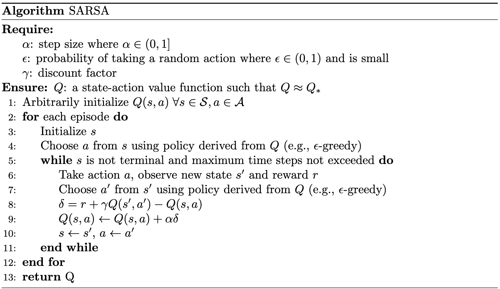
Prediction's theoretical principles extend naturally to control, as demonstrated by the mathematical parallel between TD(0) and SARSA (state-action-reward-state-action):

\[ \begin{align} \delta_{t} &= r_{t+1} + \gamma Q(s_{t+1},a_{t+1}) - Q(s_t, a_t) \label{eq:sarsa_td_error} \\ Q(s_t, a_t) &\gets Q(s_t, a_t) + \alpha \delta_{t} \;. \nonumber \end{align} \]

Despite this similarity, there is an important distinction. Prediction methods estimate the state-value function \(V_\pi(s)\) by observing transitions between states. Control methods determine optimal policies by evaluating transitions between state-action pairs. Thus, while prediction focuses solely on state values, control methods must assess each action's value within each state to enable optimal action selection. This necessitates the estimation of the action-value function \(Q_\pi(s,a)\) (as in Equation \(\eqref{eq:sarsa_td_error}\)), which represents the expected return from taking action \(a\) in state \(s\) and following policy \(\pi\) thereafter.

Because they estimate the value of state-action pairs, control methods introduce a fundamental complexity beyond that of prediction. While prediction methods use the state-value Bellman expectation equation:

\[ \begin{equation}\label{eq:sa-value} V_\pi(s) = \sum_{a \in \mathcal{A}} \pi(a \mid s) \left[ R(s,a) + \gamma \sum_{s’ \in \mathcal{S}} P(s,a,s’) V_\pi (s^\prime) \right] \;, \end{equation} \]

to estimate state values across all possible actions (see the outer summation in Equation \(\eqref{eq:sa-value}\)), control methods focus on the value of a specific action, requiring an action-selection mechanism to guide decision-making. Selecting the greedy action \(a^*\) in each state might seem like a natural approach. Until convergence, however, our current value function remains sub-optimal, and consequently, \(a^*\) only represents the best action relative to our current estimates. Therefore, to avoid prematurely settling on sub-optimal behaviors, the agent must explore by occasionally selecting actions that may appear inferior in the short term but could yield higher long-term rewards. Despite this need to explore, selecting the greedy action remains rational much of the time, as \(a^*\) represents the best action according to the agent's current knowledge. This fundamental tension between discovering new opportunities and leveraging known rewards is called the exploration vs. exploitation tradeoff. Various strategies manage this tradeoff, with the \(\epsilon\)-greedy approach being a simple yet effective method: given \(\epsilon \in [0,1]\), the agent selects a random action with probability \(\epsilon\) and the greedy action with probability \((1-\epsilon)\).

Q-learning

Q-learning is very similar to SARSA with an important, defining difference: SARSA is an on-policy algorithm while Q-learning is an off-policy algorithm. In on-policy learning the agent attempts to improve its behavior policy — the policy it uses to select actions. In off-policy learning, the agent seeks to improve a target policy — typically the optimal policy, as in Q-learning — which differs from its behavior policy. Notice that in Equation \(\eqref{eq:sarsa_td_error}\) SARSA calculates the TD error with respect to the action selected by the behavior policy, while in Equation \(\eqref{eq:q_learning_td_error}\) the TD error is calculated using the greedy action (NB the \(\max_{a’}\) operator); i.e., selecting \(a'\) without exploration (equivalent to setting \(\epsilon=0\) ):

\[ \begin{align}\label{eq:q_learning_td_error} \delta_{t} &= r_{t+1} + \gamma \max_{a’} Q(s_{t+1},a’) - Q(s_t, a_t) && && \text{cf. } \eqref{eq:sarsa_td_error} \\ Q(s_t, a_t) &\gets Q(s_t, a_t) + \alpha \delta_{t} \;. \nonumber \end{align} \]

This formulation enables Q-learning to approximate \(Q_*\) directly, while still selecting actions according to its behavior policy.

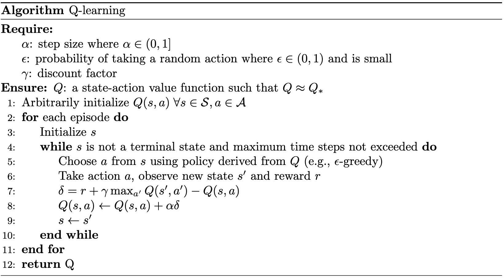SARSA and Q-learning also differ in how they handle action selection, reflecting their distinct approaches to policy evaluation and improvement. SARSA, as an on-policy algorithm, updates its value estimates using the agent's actual trajectory, which requires temporal consistency in action selection. When the agent transitions to state \(s'\) and chooses action \(a'\) following its policy (e.g., \(\epsilon\)-greedy), SARSA commits to these assignments (\(s \gets s'\), \(a \gets a'\) on line 10) to ensure the updates reflect the true behavior under the current policy. Re-selecting actions at each state via \(\epsilon\)-greedy (such as done by Q-learning on line 5) would create hypothetical trajectories divorced from actual behavior, compromising SARSA's fundamental on-policy nature.

Q-learning operates with greater independence by separating its update rule from the agent's selected actions. Instead of using the value of the actually chosen next action, Q-learning uses the maximum action-value at the next state, \(\max_{a’} Q(s’, a’)\). This decoupling means each update to \(Q(s, a)\) estimates the expected return if the agent were to act greedily in all future states, independent of its current policy. As a result, on line 5 Q-learning can freely reselect actions without compromising convergence to the optimal policy, as its updates are anchored to ideal future returns rather than actual behavior.

The effect of this difference is best illustrated by Cliff Walking, a canonical undiscounted, episodic task. The agent navigates a grid world with defined start \(s_0\) and goal \(s_G\) states by selecting from cardinal direction movements (up, down, left, right). All transitions incur a reward of -1, except for transitions into the designated “Cliff” region, which yield a reward of -100 and trigger an immediate reset to the start state.

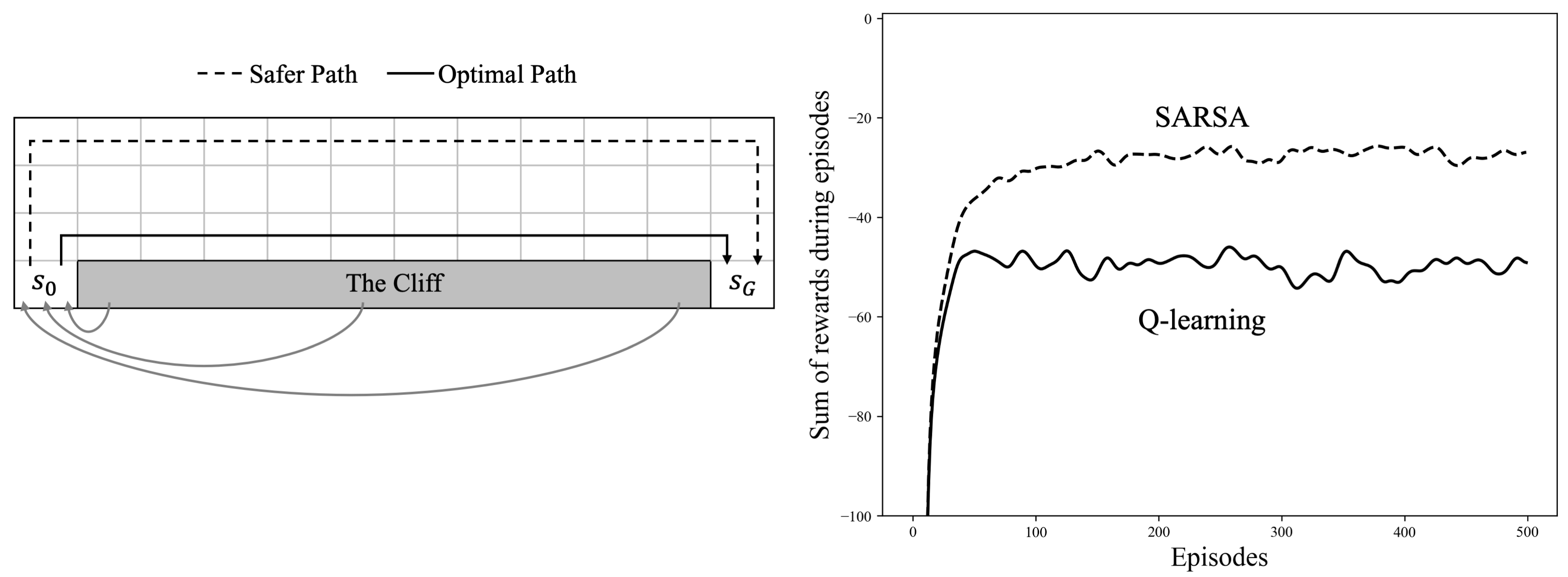The plot above demonstrates a significant behavioral divergence between SARSA and Q-learning when operating under \(\epsilon\)-greedy exploration (\(\epsilon\)=0.1). Q-learning converges to the optimal policy — traversing the path adjacent to the cliff — after an initial learning phase. However, this theoretically optimal policy is problematic in practice due to the persistent exploration mandated by \(\epsilon\)-greedy action selection, occasionally resulting in catastrophic falls. SARSA, by accounting for the effect of the random actions in its value estimation, develops a more conservative policy that favors a longer but safer route through the grid's upper region. This difference would ultimately vanish if \(\epsilon\) were annealed toward zero.

Convergence

Both SARSA and Q-learning adhere to the Generalized Policy Iteration (GPI) framework, using TD learning for policy evaluation and \(\epsilon\)-greedy action selection for improvement. Under conditions common in stochastic approximation theory, Q-learning converges to an optimal policy and action-value function, provided that each state–action pair is visited infinitely often and:

\[ \begin{align*} \sum_{n=1}^\infty \alpha_n &= \infty \;, && \sum_{n=1}^\infty \alpha^2_n < \infty \;, \end{align*} \]

where the first condition ensures steps remain sufficiently large to overcome initial conditions and random fluctuations, allowing meaningful value estimate adjustments if, for example, the initial estimate is far from the true value. The second condition ensures convergence by gradually reducing step sizes until updates effectively cease; without this, persistent random fluctuations would prevent stabilization to an optimal value.

For on-policy methods like SARSA, which rely on a single policy for both exploration and improvement, these conditions alone do not guarantee convergence to an optimal policy. With constant \(\epsilon\), SARSA converges to a near-optimal policy that continues to explore. However, SARSA converges to the optimal policy with probability 1 when the policy becomes greedy in the limit (e.g., if \(\epsilon = 1/t\)).

The Difference Between SARSA and Q-learning When \(\epsilon=0\)

When \(\epsilon = 0\) and both methods use a greedy policy, SARSA and Q-learning use the same update target, since SARSA’s next action \(a_{t+1}\) is \(\arg\max_{a’} Q(s_{t+1},a’)\). Given the same sequence of transitions, they perform identical updates. Meaningful behavioral differences between SARSA and Q-learning arise when the behavior policy is stochastic (e.g., \(\epsilon > 0\)).

References

Reinforcement Learning: An Introduction (2018)

Richard S. Sutton and Andrew G. Barto

Artificial Intelligence: A Modern Approach, 4th edition (2020)

Stuart Russell and Peter Norvig

Reinforcement Learning: An Introduction (1998)

Richard S. Sutton and Andrew G. Barto

Model-Free Control, Lectures on Reinforcement Learning (2015)

David Silver