Cross-Entropy Method

Published February 3, 2026

The Importance Sampling and KL Divergence notes are optional but recommended background reading.

Global optimization of a scalar performance function \(V(\cdot\,;s): \mathcal{A} \to \mathbb{R}\) over an action space \(\mathcal{A}\), conditioned on a fixed state \(s\in\mathcal{S}\), can be expressed as:

\[ \begin{equation}\label{eq:global-optimization} V^*(s) = \sup_{a \in \mathcal{A}} V(a;s), \qquad a^*(s) \in \arg\max_{a \in \mathcal{A}} V(a;s) \;. \end{equation} \]

This formulation, however, relies on the supremum operator, which is purely extremal. It defines the optimal value but provides no information regarding the global structure of \(V(\cdot\,;s)\) away from the maximizer \(a^*(s)\). Furthermore, the maximizer need not depend continuously on perturbations to \(V(\cdot\,;s)\). Consequently, this objective admits no obvious incremental decomposition or controlled path from suboptimal actions toward \(a^*(s)\).

An iterative method can be constructed by replacing the extremal objective with an aggregate measure over the action space. Specifically, we can consider the “size” of the superlevel set \(\{ a \in \mathcal{A} : V(a;s) \ge \gamma \}\) for a threshold \(\gamma \in \mathbb{R}\), by defining a reference measure. Let \(A \sim \mu(\cdot\mid s)\), where \(\mu(\cdot\mid s)\) is a fixed reference probability measure on \(\mathcal{A}\) (conditioned on \(s\)). The probability of observing performance exceeding \(\gamma\) is defined as:

\[ \begin{equation*} \ell_s(\gamma) = \mathbb{P}_{\mu(\cdot\mid s)}(V(A;s) \ge \gamma) = \mathbb{E}_{\mu(\cdot\mid s)} \left[ \mathbf{1}_{\{V(A;s) \ge \gamma\}} \right]. \end{equation*} \]

The function \(\ell_s(\gamma)\) is non-increasing by construction — raising the threshold \(\gamma\) guarantees that the probability of exceeding the threshold does not increase. Since \(\ell_s(\gamma)>0\) holds if and only if \(\mu(\{a\in\mathcal A:V(a;s)\ge \gamma\}\mid s)>0\), the set of feasible thresholds

\[ \begin{equation*} \Gamma_s = \{ \gamma \in \mathbb{R} : \ell_s(\gamma) > 0 \} \end{equation*} \]

consists of all \(\gamma\) for which \(V(\cdot\,;s)\) attains values at least \(\gamma\) on a subset of \(\mathcal{A}\) with positive \(\mu(\cdot\mid s)\)-mass. For any \(\gamma>\sup_{a\in\mathcal A}V(a;s)\), this condition fails and \(\ell_s(\gamma)=0\). The least upper bound of \(\Gamma_s\) defines the \(\mu(\cdot\mid s)\)-essential supremum:

\[ \begin{equation*} V^*_{\mu}(s) := \sup \{ \gamma : \ell_s(\gamma) > 0 \} = \operatorname*{ess\,sup}_{\mu(\cdot\mid s)} V(\cdot\,;s) \;. \end{equation*} \]

If, in addition, \(\mu(\cdot\mid s)\) assigns positive mass to sets attaining values arbitrarily close to the global supremum:

\[ \begin{equation*} \mu\bigl(\{a\in\mathcal A:V(a;s)\ge \sup_{x\in\mathcal A}V(x;s)-\varepsilon\}\mid s\bigr)>0 \quad\text{for all }\varepsilon>0, \end{equation*} \]

then:

\[ \begin{equation*} \sup_{a\in\mathcal A}V(a;s)=V^*_{\mu}(s)=\sup\{\gamma:\ell_s(\gamma)>0\} \;. \end{equation*} \]

In contrast to Equation \(\eqref{eq:global-optimization}\), here the essential supremum serves only to characterize \(V^*(s)\); it is not an optimization primitive. This reformulation forms the foundation of the Cross-Entropy Method (CEM) — the extremal objective, which provides no graded notion of progress away from the maximizer, is substituted with a family of statistical quantities \(\{\ell_s(\gamma)\}_{\gamma}\) that characterize how the reference measure \(\mu(\cdot\mid s)\) allocates mass to high-value regions of the action space.

Feasibility of Superlevel Sets Surrogate

Rewriting Equation \(\eqref{eq:global-optimization}\) in terms of superlevel sets provides a scalar surrogate for action maximization, in which progress toward the optimum is measured by increasing a threshold \(\gamma\) rather than directly improving \(V(a;s)\). The feasibility of this surrogate, however, depends on whether the associated exceedance probability can be estimated reliably as \(\gamma\) approaches \(V^*(s)\).

The accuracy of estimations for \(\ell_s(\gamma)\) can be quantified by the variance of the Monte Carlo estimator. Let \(A_1,\dots,A_N\sim\mu(\cdot\mid s)\) be independent samples and define:

\[ \begin{equation*} X_k = \mathbf{1}_{\{V(A_k;s)\ge\gamma\}}, \qquad \hat{\ell}^{\mathrm{MC}}_N(\gamma;s) = \frac{1}{N}\sum_{k=1}^N X_k . \end{equation*} \]

The variance of this estimator is:

\[ \begin{align} \mathrm{Var}\!\left(\hat{\ell}^{\mathrm{MC}}_N(\gamma;s)\right) &= \mathrm{Var}\!\left(\frac{1}{N}\sum_{k=1}^N X_k\right) \nonumber \\ &= \frac{1}{N^2}\sum_{k=1}^N \mathrm{Var}(X_k) && \text{by independence of samples} \nonumber \\ &= \frac{1}{N}\,\ell_s(\gamma)\bigl(1-\ell_s(\gamma)\bigr) && \text{by definition of Bernoulli variance} \label{eq:variance}. \end{align} \]

However, since \(\gamma\) is typically chosen so that \(\ell_s(\gamma)\) is small (i.e., high value actions are rare under \(\mu(\cdot\mid s)\)), an absolute variance can be small even when the estimator has large error relative to \(\ell_s(\gamma)\). Dividing by \(\ell_s(\gamma)^2\) yields the more informative relative variance:

\[ \begin{align} \frac{\mathrm{Var}\!\left(\hat{\ell}^{\mathrm{MC}}_N(\gamma;s)\right)}{\ell_s(\gamma)^2} &= \frac{\frac{1}{N}\,\ell_s(\gamma)\bigl(1-\ell_s(\gamma)\bigr)}{\ell_s(\gamma)^2} && \text{by Equation } \eqref{eq:variance} \nonumber \\ &= \frac{1}{N}\,\frac{1-\ell_s(\gamma)}{\ell_s(\gamma)} \nonumber \\ &\approx \frac{1}{N\,\ell_s(\gamma)} && \text{for small } \ell_s(\gamma) \;. \label{eq:relative-variance} \end{align} \]

Thus, as \(\ell_s(\gamma)\) decreases, maintaining fixed relative accuracy requires a number of samples proportional to \(1/\ell_s(\gamma)\).

Sampling Distributions Concentrated on High-Value Actions

By Equation \(\eqref{eq:relative-variance}\), estimation of \(\ell_s(\gamma)\) under the nominal measure \(\mu(\cdot\mid s)\) becomes unstable as \(\gamma\) approaches \(V^*(s)\) (assuming \(\ell_s(\gamma)\) is small). CEM therefore replaces direct sampling from \(\mu(\cdot\mid s)\) with a sequence of alternative sampling measures that reallocate probability mass toward high-value regions of the action space.

Assume \(\mu(\cdot\mid s)\) has density or mass function \(f(\cdot;\mathbf{u})\) on \(\mathcal{A}\), drawn from a family parameterized by \(\mathbf{u}\). The exceedance probability admits the integral representation:

\[ \begin{equation*} \ell_s(\gamma) = \int \mathbf{1}_{\{V(a;s)\ge\gamma\}} f(a;\mathbf{u})\,da . \end{equation*} \]

Let \(g\) be an alternative density or mass function on \(\mathcal{A}\) used for sampling. Require that \(g(a)>0\) whenever \(f(a;\mathbf{u})>0\) and \(V(a;s)\ge\gamma\). Under this condition, \(\ell_s(\gamma)\) can be expressed as an expectation under \(g\) via importance sampling:

\[ \begin{equation*} \ell_s(\gamma) = \mathbb{E}_g\!\left[ \mathbf{1}_{\{V(A;s)\ge\gamma\}} \frac{f(A;\mathbf{u})}{g(A)} \right]. \end{equation*} \]

Given independent samples \(A_1,\dots,A_N\sim g\), define the unbiased estimator:

\[ \begin{equation*} \hat{\ell}_N(\gamma;s) = \frac{1}{N}\sum_{k=1}^N \mathbf{1}_{\{V(A_k;s)\ge\gamma\}} \frac{f(A_k;\mathbf{u})}{g(A_k)} = \frac{1}{N}\sum_{k=1}^N Y(A_k). \end{equation*} \]

For any admissible sampling density \(g\), the importance sampling identity preserves the value of \(\ell_s(\gamma)\) (\(\mathbb{E}_g[Y(A)] = \ell_s(\gamma)\)). However, the choice does affect the variance of the importance sampling estimator. Specifically, for an unbiased Monte Carlo estimator, the mean-squared error is equal to variance. Smaller variance therefore yields higher accuracy for fixed sample size \(N\). The limiting case is \(\mathrm{Var}_g(\hat{\ell}_N(\gamma;s))=0\), which corresponds to exact recovery of \(\ell_s(\gamma)\) from finitely many samples. Since \(\hat{\ell}_N(\gamma;s)\) is an empirical average of i.i.d. random variables its variance is defined as:

\[ \begin{align*} \mathrm{Var}_g(\hat{\ell}_N(\gamma;s)) = \frac{1}{N}\,\mathrm{Var}_g(Y(A)) && \text{by the variance-of-the-sample-mean identity.} \end{align*} \]

Zero variance of the estimator therefore requires \(\mathrm{Var}_g(Y(A))=0\). A square-integrable random variable has zero variance if and only if it is constant \(g\)-almost surely. Because the importance sampling estimator is unbiased, the constant must equal \(\ell_s(\gamma)\):

\[ \begin{equation}\label{eq:zero-variance} Y(a) = \mathbf{1}_{\{V(a;s)\ge\gamma\}} \frac{f(a;\mathbf{u})}{g(a)} = \ell_s(\gamma) \qquad \text{for all } a \text{ with } g(a)>0 . \end{equation} \]

Solving Equation \(\eqref{eq:zero-variance}\) yields a unique density:

\[ \begin{equation}\label{eq:zero-variance-measure} g^*(a) = \frac{\mathbf{1}_{\{V(a;s)\ge\gamma\}} f(a;\mathbf{u})}{\ell_s(\gamma)} . \end{equation} \]

KL Projection

While the ideal sampling strategy \(g^*\) restricts support entirely to the success region, its value depends on the unknown quantity \(\ell_s(\gamma)\) (Equation \(\eqref{eq:zero-variance-measure}\)) and is thus not directly implementable. It can, however, serve as a reference distribution for constructing parametric sampling families.

Let \(\mathcal{F} = \{ f(\cdot;\mathbf{v}) : \mathbf{v} \in \mathcal{V} \}\) be a parametric family of tractable sampling distributions on \(\mathcal{A}\). CEM approximates \(g^*\) by the KL projection of \(g^*\) onto \(\mathcal{F}\):

\[ \begin{align*} \mathbf{v}^* &= \arg\min_{\mathbf{v}\in\mathcal{V}} D_{\mathrm{KL}}(g^* \,\|\, f(\cdot;\mathbf{v})) \\ &= \arg\min_{\mathbf{v}\in\mathcal{V}} \int g^*(a)\ln\frac{g^*(a)}{f(a;\mathbf{v})}\,da \\ &= \arg\min_{\mathbf{v}\in\mathcal{V}} \int g^*(a)\ln g^*(a)\,da - \int g^*(a)\ln f(a;\mathbf{v})\,da \\ &= \arg\max_{\mathbf{v}\in\mathcal{V}} \int g^*(a)\ln f(a;\mathbf{v})\,da \;. \\ \end{align*} \]

Substituting the expression for \(g^*\) from Equation \(\eqref{eq:zero-variance-measure}\) yields:

\[ \begin{align*} \int g^*(a)\ln f(a;\mathbf{v})\,da &= \int \frac{\mathbf{1}_{\{V(a;s)\ge\gamma\}} f(a;\mathbf{u})}{\ell_s(\gamma)} \ln f(a;\mathbf{v})\,da \\ &= \frac{1}{\ell_s(\gamma)} \int \mathbf{1}_{\{V(a;s)\ge\gamma\}} f(a;\mathbf{u}) \ln f(a;\mathbf{v})\,da . \end{align*} \]

Dropping the constant factor \(1/\ell_s(\gamma)\) and writing the remaining integral as an expectation under the reference density \(f(\cdot;\mathbf{u})\) gives the equivalent optimization problem:

\[ \begin{equation}\label{eq:ce-stochastic-program} \mathbf{v}^* = \arg\max_{\mathbf{v}\in\mathcal{V}} \mathbb{E}_{\mathbf{u}}\!\left[ \mathbf{1}_{\{V(A;s)\ge\gamma\}} \ln f(A;\mathbf{v}) \right]. \end{equation} \]

The expectation in Equation \(\eqref{eq:ce-stochastic-program}\) is approximated via Monte Carlo integration. Given samples \(A_1,\dots,A_N \sim f(\cdot;\mathbf{u})\), define the empirical objective:

\[ \begin{equation*} \hat{J}(\mathbf{v}) = \frac{1}{N}\sum_{k=1}^N \mathbf{1}_{\{V(A_k;s)\ge\gamma\}} \ln f(A_k;\mathbf{v}). \end{equation*} \]

The resulting maximization problem reduces to maximum-likelihood estimation over the elite subset — the samples for which the respective objective values satisfy \(V(A_k;s)\ge\gamma\).

Objective Maximization

Let \(\mathcal{I} = \{ k : V(A_k;s) \ge \gamma \}\) denote the index set of elite samples. Maximization of \(\hat{J}(\mathbf{v})\) is equivalent to maximum-likelihood estimation over the elite subset:

\[ \begin{equation}\label{eq:mle-elite} \hat{\mathbf{v}} \in \arg\max_{\mathbf{v} \in \mathcal{V}} \sum_{k \in \mathcal{I}} \ln f(A_k; \mathbf{v}). \end{equation} \]

For a differentiable density, this objective admits gradient-based solution methods. However, CEM typically restricts the model class \(\mathcal{F}\) to the natural exponential family, since the MLE then admits a closed form solution.

For discrete control problems where \(\mathcal{A} = \{0, 1\}^d\), for example, the sampling distribution is often chosen as a multivariate Bernoulli with independent components, parameterized by \(\mathbf{p} \in [0,1]^d\). The probability mass function is:

\[ \begin{equation*} f(\mathbf{a}; \mathbf{p}) = \prod_{j=1}^d p_j^{a_j} (1-p_j)^{1-a_j}. \end{equation*} \]

The log-likelihood \(\mathcal{L}(\mathbf{p})\) decomposes into a sum over the components:

\[ \begin{align*} \mathcal{L}(\mathbf{p}) &= \sum_{k \in \mathcal{I}} \ln \left( \prod_{j=1}^d p_j^{A_{k,j}} (1-p_j)^{1-A_{k,j}} \right) \\ &= \sum_{k \in \mathcal{I}} \sum_{j=1}^d \left( A_{k,j} \ln p_j + (1-A_{k,j}) \ln(1-p_j) \right) \\ &= \sum_{j=1}^d \left( \ln p_j \sum_{k \in \mathcal{I}} A_{k,j} + \ln(1-p_j) \sum_{k \in \mathcal{I}} (1-A_{k,j}) \right). \end{align*} \]

To find the optimal parameter \(\hat{p}_j\), differentiate with respect to \(p_j\) and set the gradient to zero:

\[ \begin{align} \frac{\partial \mathcal{L}}{\partial p_j} &= \frac{1}{p_j} \sum_{k \in \mathcal{I}} A_{k,j} - \frac{1}{1-p_j} \sum_{k \in \mathcal{I}} (1-A_{k,j}) = 0 \nonumber \\ (1-p_j) \sum_{k \in \mathcal{I}} A_{k,j} &= p_j \sum_{k \in \mathcal{I}} (1-A_{k,j}) \nonumber \\ \sum_{k \in \mathcal{I}} A_{k,j} - p_j \sum_{k \in \mathcal{I}} A_{k,j} &= p_j |\mathcal{I}| - p_j \sum_{k \in \mathcal{I}} A_{k,j} \nonumber \\ \sum_{k \in \mathcal{I}} A_{k,j} &= p_j |\mathcal{I}|. \label{eq:bernoulli-deriv} \end{align} \]

Solving Equation \(\eqref{eq:bernoulli-deriv}\) for \(p_j\) yields the update rule:

\[ \begin{equation*} \hat{p}_j = \frac{1}{|\mathcal{I}|} \sum_{k \in \mathcal{I}} A_{k,j}. \end{equation*} \]

Thus, the analytic solution to the empirical maximization problem is simply the sample mean of the elite action vectors.

Continuous Action Case

For continuous control with \(\mathcal{A} = \mathbb{R}^d\), the multivariate Gaussian is a canonical choice for the sampling family \(\mathcal{F}\). For a fixed state \(s\in\mathcal{S}\), let

\[ \begin{equation*} f(\cdot;\mathbf{v}) = \mathcal{N}(\cdot;\mu,\Sigma), \qquad \mathbf{v}=(\mu,\Sigma), \end{equation*} \]

where \(\mu\in\mathbb{R}^d\) and \(\Sigma\in\mathbb{S}_{++}^d\). At iteration \(t\), draw \(A_1,\dots,A_N\sim \mathcal{N}(\mu_{t-1},\Sigma_{t-1})\), evaluate \(\{V(A_k;s)\}_{k=1}^N\), and form the elite index set \(\mathcal{I}_t=\{k:V(A_k;s)\ge \gamma\}\).

The CEM update maximizes the empirical elite log-likelihood (Equation \(\eqref{eq:mle-elite}\)) which, for the Gaussian family, admits a closed-form maximum-likelihood solution. Specifically, the updated mean and covariance are the empirical moments of the elite actions:

\[ \begin{equation*} \hat{\mu}_t = \frac{1}{|\mathcal{I}_t|}\sum_{k\in\mathcal{I}_t} A_k, \qquad \hat{\Sigma}_t = \frac{1}{|\mathcal{I}_t|}\sum_{k\in\mathcal{I}_t}(A_k-\hat{\mu}_t)(A_k-\hat{\mu}_t)^\top. \end{equation*} \]

Stabilized Updates

Stability of the parameter update depends critically on the threshold \(\gamma\) and on the numerical conditioning of the resulting maximum-likelihood fit. A fixed threshold yields two degenerate regimes for the empirical objective \(\hat{J}(\mathbf{v})\). If \(\gamma\) is too large, the elite set is empty, the objective equals zero, and the maximizer is undefined. If \(\gamma\) is too small, the elite set equals the full sample, and the likelihood maximization returns parameters close to the sampling distribution that generated the data, producing little or no concentration of mass toward high-value actions.

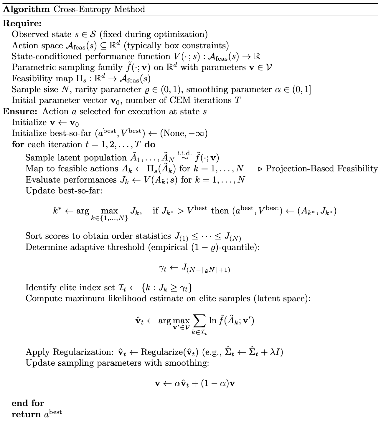
CEM avoids these degeneracies by selecting the threshold adaptively to retain approximaltey a fixed fraction (accounting for ties e.g., if multiple samples have identical performance values at the threshold) of samples. Fix a rarity parameter \(\varrho\in(0,1)\). At iteration \(t\), draw \(A_1,\dots,A_N\sim f(\cdot;\mathbf{v}_{t-1})\) and form the order statistics \(V_{(1)}\le \cdots \le V_{(N)}\) of the values \(V(A_k;s)\). Define the threshold as the empirical \((1-\varrho)\)-quantile:

\[ \begin{equation*} \gamma_t = V_{(N-\lceil \varrho N \rceil + 1)}. \end{equation*} \]

Let \(\mathcal{I}_t = \{k : V(A_k;s)\ge \gamma_t\}\) denote the elite index set. The parameter update is then obtained by maximum-likelihood estimation over the elite subset:

\[ \begin{equation*} \hat{\mathbf{v}}_t \in \arg\max_{\mathbf{v}\in\mathcal{V}} \sum_{k=1}^N \mathbf{1}_{\{V(A_k;s)\ge \gamma_t\}} \ln f(A_k;\mathbf{v}). \end{equation*} \]

In continuous-action settings, adaptive levels alone do not prevent premature concentration: even with fixed elite fraction, the elite actions may be tightly clustered, and maximum-likelihood fitting of expressive families can yield overly concentrated or ill-conditioned dispersion parameters (e.g., near-singular covariances under Gaussian sampling). CEM therefore uses stabilized updates that combine adaptive thresholding with additional mechanisms to control the rate of concentration.

For Gaussian sampling with \(\mathbf{v}=(\mu,\Sigma)\), covariance regularization is a standard stabilization:

\[ \begin{equation*} \hat{\Sigma}_t \leftarrow \hat{\Sigma}_t + \lambda I, \qquad \lambda>0, \end{equation*} \]

applied after computing the elite MLE and before committing to the next iterate. Finally, a smoothed update limits step size by blending the new estimate with the previous parameters. Assuming the the parameter space \(\mathcal{V}\) is convex:

\[ \begin{equation*} \mathbf{v}_t = \alpha \hat{\mathbf{v}}_t + (1-\alpha)\mathbf{v}_{t-1}, \qquad \alpha\in(0,1] \;. \end{equation*} \]

Together, adaptive thresholding ensures a reliable elite signal, while regularization and smoothing prevent premature collapse and improve robustness of the parameter update in continuous-action settings.

Constraints and Feasibility Handling

In real-world settings, admissible actions are frequently restricted to a feasible set \(\mathcal{A}_{\mathrm{feas}}(s)\subseteq\mathcal{A}\) (e.g., actuator limits, safety constraints, or state-dependent constraints). Since CEM constructs and updates a sampling distribution over actions, feasibility must be enforced either at the level of the sampling map, the sampling distribution, or the objective used to define elites. Several standard mechanisms are used.

Reparameterization or Projection into \(\mathcal{A}_{\mathrm{feas}}(s)\)

Actions are sampled in an unconstrained latent space \(\tilde{\mathcal{A}}=\mathbb{R}^d\) and mapped into the feasible set via a deterministic feasibility map \(\Pi_s:\tilde{\mathcal{A}}\to\mathcal{A}_{\mathrm{feas}}(s)\), with \(A=\Pi_s(\tilde{A})\) and \(\tilde{A}\sim \tilde{f}(\cdot;\mathbf{v})\). For example, \(\Pi_s\) may be defined as a metric projection:

\[ \begin{equation*} \Pi_s(\tilde{a}) \in \arg\min_{a\in\mathcal{A}_{\mathrm{feas}}(s)} \|a-\tilde{a}\| . \end{equation*} \]

This construction enforces feasibility by design, at the cost of distorting the effective sampling distribution near the boundary of \(\mathcal{A}_{\mathrm{feas}}(s)\).

Rejection of Infeasible Samples

Actions are sampled directly from \(f(\cdot;\mathbf{v})\) on \(\mathcal{A}\) and infeasible draws are discarded until a feasible set of size \(N\) is obtained. This preserves the original parameterization on \(\mathcal{A}\) but becomes inefficient when \(\mathbb{P}_{f(\cdot;\mathbf{v})}(A\in\mathcal{A}_{\mathrm{feas}}(s))\) is small, which can increase variance and destabilize updates.

Penalized Objectives

Feasibility is enforced implicitly by modifying the performance function used to form elites. Given a violation measure \(\phi(a;s)\ge 0\) (with \(\phi(a;s)=0\) for \(a\in\mathcal{A}_{\mathrm{feas}}(s)\)), define a penalized score:

\[ \begin{equation*} \tilde{V}(a;s) = V(a;s) - \kappa\,\phi(a;s), \qquad \kappa>0. \end{equation*} \]

CEM is then applied to \(\tilde{V}\) in place of \(V\). The resulting behavior depends on the penalty weight: if \(\kappa\) is too small, infeasible actions may remain elite; if \(\kappa\) is too large, the search may become dominated by constraint satisfaction rather than task performance.

Truncated Sampling Distributions

When tractable, sampling is performed from a distribution restricted to the feasible set:

\[ \begin{equation*} f_{\mathrm{tr}}(a;\mathbf{v},s) = \frac{f(a;\mathbf{v})\,\mathbf{1}_{\{a\in\mathcal{A}_{\mathrm{feas}}(s)\}}} {\int f(\bar{a};\mathbf{v})\,\mathbf{1}_{\{\bar{a}\in\mathcal{A}_{\mathrm{feas}}(s)\}}\,d\bar{a}} . \end{equation*} \]

This enforces feasibility without rejection, but complicates both sampling and parameter estimation, since the normalization depends on \((\mathbf{v},s)\) and maximum-likelihood updates must respect the truncation.

These mechanisms trade off feasibility guarantees, sampling efficiency, and fidelity of the induced sampling distribution. In practice, simple box constraints are commonly handled via reparameterization or projection, whereas complex constraints may require penalty formulations or truncated sampling.

Constrained CEM vs Constrained RL

CEM-based constraint handling can appear similar to constrained RL as both ultimately rely on the same high-level mechanisms (projection, rejection, penalties, or truncation). The fundamental distinction is not the mechanism itself, but where constraints are enforced. In the RL setting, constraints must be satisfied by a learned policy across a distribution of states, and feasibility typically emerges statistically through training and generalization.

CEM, by contrast, is applied as an online constrained optimization procedure at the current state \(s\): feasibility can be imposed directly on the sampled candidate actions (e.g., by projection or truncated sampling), ensuring that the actions considered — and therefore the elites driving the update — lie in \(\mathcal{A}_{\mathrm{feas}}(s)\). Consequently, constraint satisfaction can be guaranteed at execution time without requiring differentiability of the dynamics, reward, or constraints, and without relying on asymptotic training behavior (unless using penalized objectives as the sole constraint mechanism). The tradeoff is computational — CEM expends online sampling effort to obtain feasible high-value actions, whereas constrained RL seeks a policy that is cheap to evaluate at runtime but is typically harder to train robustly under hard constraints.

References

The Cross-Entropy Method for Optimization (2013)

Zdravko Botev, Dirk Kroese, Reuven Rubinstein, and Pierre L'ecuyer

The Cross-Entropy Method: A Unified Approach to Rare Event Simulation and Stochastic Optimization (accessed 2026)

Dirk P. Kroese and Reuven Y. Rubinstein