Value Functions and Policies
Revised June 11, 2024
The Markov Decision Processes note is optional but recommended background reading.
In a Markov Decision Process (MDP), a decision-making agent seeks to maximize the sum of its discounted rewards. Expressed slightly differently, the agent prioritizes visiting states with the highest expected return. Consider the figure below. Assuming all other factors are equal, the agent should prefer state \(s_3\) over \(s_1\) because \(s_3\) has a higher expected return:
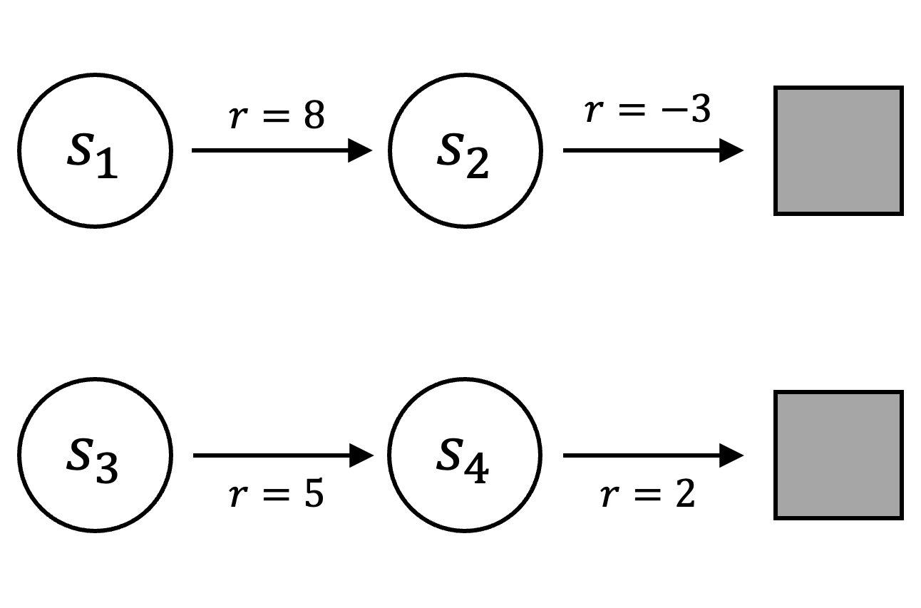 |
\[ \begin{align*} V(s_1) &= 8 + (0.9 \cdot -3) = 5.3 && \text{with } \gamma = 0.9 \\ V(s_3) &= 5 + (0.9 \cdot 2) = 6.8 \end{align*} \]
A state's value, or more precisely its expected return, can be formalized with the value function. Because transitioning between states requires actions, the value function is defined with respect to a sequence of actions called a policy. In the MDP below, for example, the value of \(s_0\) depends on the agent selecting either action \(a=0\) or \(a=1\):
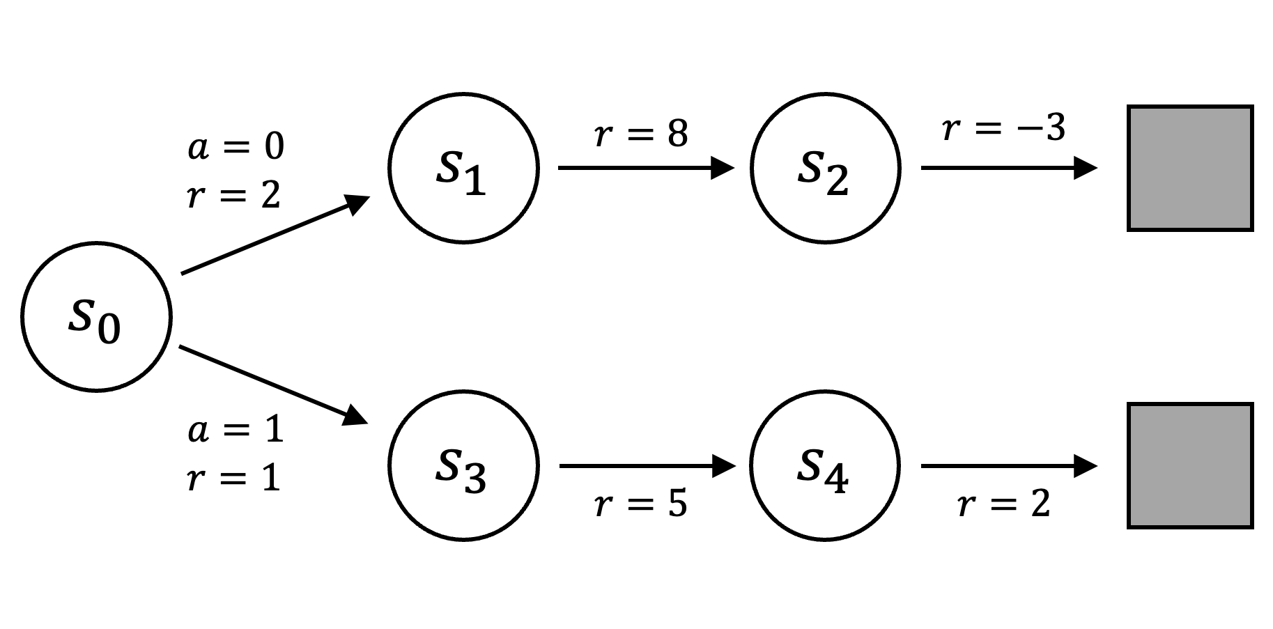 |
| Note that the transitions between all states require an action, but because only one action is available in \(s_1, s_2, s_3,\) and \(s_4\), we omit the selected action to simplify notation. |
\[ \begin{align*} V(s_0 \mid a_0) = 2 + (0.9 \cdot 8) + (0.9*0.9 \cdot -3) = 6.77 \\ V(s_0 \mid a_1) = 1 + (0.9 \cdot 5) + (0.9*0.9 \cdot 2) = 7.12 \end{align*} \]
Policies can be categorized by their nature (deterministic or stochastic) and by their temporal behavior (stationary or non-stationary). A deterministic policy maps each state to a specific action \(\pi: s \rightarrow a\). A stochastic policy, by contrast, is a conditional density; it maps a state to a probability distribution over actions \(\pi(a \mid s) = \mathbb{P}[a_t = a \mid s_t = s]\). A stationary policy is time-invariant, selecting actions based solely on the current state, such that \(a_t \sim \pi(\cdot \mid s_t)\) holds for all timesteps \(t\). A non-stationary policy permits temporal variation in action selection, formally expressed as \(\pi_i \neq \pi_j\) for any timesteps \(i \neq j\). This means that given the same state, a non-stationary policy may select different actions depending on when the decision is made.
There are two types of value functions. The state-value function quantifies the value of a state \(s\) under a policy \(\pi\):
\[ \begin{equation*} V_\pi (s) = \mathbb{E}_\pi [G_t \mid s_t = s] \; , \end{equation*} \]
where \(G_t = \sum_{k=0}^{H} \gamma^k r_{t+k+1}\) represents the discounted sum of future rewards from time \(t\) (for more details, refer to the MDP note).
The action-value function quantifies the value of taking action \(a\) in state \(s\) under policy \(\pi\):
\[ \begin{equation}\label{eq:action-value-function} Q_\pi (s,a) = \mathbb{E}_\pi [G_t \mid s_t = s, a_t = a] \;. \end{equation} \]
Informally, the action-value function gives the expected return when taking action \(a\) in state \(s\) and following policy \(\pi\) thereafter.
The Bellman Expectation Equations
The Bellman equation provides a recursive decomposition of the value function, offering a structured method to evaluate the value of a state. It expresses a state's value in terms of its immediate reward and the discounted value of its successor state:
\[ \begin{align} V_\pi (s) &= \mathbb{E}_\pi [G_t \mid s_t = s] \nonumber \\ &= \mathbb{E}_\pi \Bigg[ \sum_{k=0}^{\infty} \gamma^k r_{t+k+1} \mid s_t = s \Bigg] \nonumber \\ &= \mathbb{E}_\pi [r_{t+1} + \gamma r_{t+2} + \gamma^2 r_{t+3} + \dots \mid s_t = s] \nonumber \\ &= \mathbb{E}_\pi [r_{t+1} + \gamma(r_{t+2} + \gamma r_{t+3} + …) \mid s_t = s] \nonumber \\ &= \mathbb{E}_\pi [r_{t+1} + \gamma G_{t+1} \mid s_t = s] \nonumber \\ &= \mathbb{E}_\pi [r_{t+1} + \gamma V_\pi (s_{t+1}) \mid s_t = s] \label{eq:immediate-plus-future} \;. \end{align} \]
This formulation separates the immediate reward from the (more uncertain) future rewards. However, as outlined in the MDP note, transitions between states can be probabilistic due to the environment, the policy, or both. To account for this stochasticity, we modify Equation \(\eqref{eq:immediate-plus-future}\) using the MDP’s constituent elements, resulting in the state-value Bellman expectation equation:
\[ \begin{align} V_\pi (s) &= \mathbb{E}_\pi [r_{t+1} + \gamma V_\pi (s_{t+1}) \mid s_t = s] \nonumber \\ &= \sum_{a \in \mathcal{A}} \pi(a \mid s) \mathbb{E} \big[r_{t+1} + \gamma V_\pi(s_{t+1}) \mid s_t=s, a_t=a \big] \nonumber \\ &= \sum_{a \in \mathcal{A}} \pi(a \mid s) \bigg( R(s,a) + \gamma \sum_{s’ \in \mathcal{S}} P(s,a,s’) V_\pi (s’) \bigg) \label{eq:sv-bellman} \;. \end{align} \]
Because we informally defined the action-value function as the expected return when taking action \(a\) in state \(s\) and then following policy \(\pi\), we can similarly extend Equation \(\eqref{eq:action-value-function}\) to derive the action-value Bellman expectation equation:
\[ \begin{align} Q_\pi (s,a) &= \mathbb{E}[r_{t+1} + \gamma V_\pi(s_{t+1}) \mid s_t = s, a_t = a] \label{eq:av_bellman} \nonumber \\ &= R(s,a) + \gamma \sum_{s’ \in \mathcal{S}} P(s,a,s’) V_\pi (s’) \nonumber \\ &= R(s,a) + \gamma \sum_{s’ \in \mathcal{S}} P(s,a,s’) \left( \sum_{a’ \in \mathcal{A}} \pi(a’ \mid s’) Q_\pi (s’,a’) \right) \label{eq:av-bellman} \;. \end{align} \]
Solving the Bellman expectation Equations \(\eqref{eq:sv-bellman}\) and \(\eqref{eq:av-bellman}\) is straightforward because the policy is fixed. We are not seeking to identify optimal actions or improve the policy; rather, we want to determine the value of a specific state or state-action pair given a static policy \(\pi\). A fixed policy reduces an MDP to a Markov Reward Process (MRP). An MRP is a special case of a Markov chain, a memoryless stochastic process characterized by a sequence of random states \(s_1, s_2, \dots\), satisfying the Markov property. A Markov chain is defined by a tuple \(\mathcal{M} = \langle \mathcal{S}, P \rangle\). An MRP extends a Markov chain by associating rewards with state transitions and is defined by \(\mathcal{M} = \langle \mathcal{S}, P, R, \gamma \rangle\). A fixed policy induces an MRP from an MDP because the agent's sequence of observed states and rewards is entirely governed by the policy \(\pi\).
In an MRP, the Bellman expectation equation can be expressed in vector and matrix form to represent rewards, values, and transition probabilities under a fixed policy \(\pi\):
\[ \begin{equation}\label{eq:bellman_matrix} \mathbf{v}_\pi = \mathbf{r}_\pi + \gamma P_\pi \mathbf{v}_\pi \;. \end{equation} \]
Expanding this into matrix notation:
\[ \begin{equation} \nonumber \begin{bmatrix} v_{1} \\ v_{2} \\ \vdots \\ v_{n} \end{bmatrix} = \begin{bmatrix} r_\pi(1) \\ r_\pi(2) \\ \vdots \\ r_\pi(n) \end{bmatrix} + \gamma \begin{bmatrix} P_\pi({1,1}) & P_\pi({1,2}) & \cdots & P_\pi({1,n}) \\ P_\pi({2,1}) & P_\pi({2,2}) & \cdots & P_\pi({2,n}) \\ \vdots & \vdots & \ddots & \vdots \\ P_\pi({n,1}) & P_\pi({n,2}) & \cdots & P_\pi({n,n}) \end{bmatrix} \begin{bmatrix} v_{1} \\ v_{2} \\ \vdots \\ v_{n} \end{bmatrix} \end{equation} \]
Here, \(\mathbf{r}_\pi\) represents the expected rewards and \(P_\pi\) represents the state transition probabilities under policy \(\pi\):
\[ \begin{equation*} r_\pi(s) = \sum_{a \in \mathcal{A}} \pi(a \mid s) R(s, a) \quad \text{and} \quad P_\pi(s, s’) = \sum_{a \in \mathcal{A}} \pi(a \mid s) P(s, a, s’) \;. \end{equation*} \]
Notice that Equation \(\eqref{eq:bellman_matrix}\) is a linear equation that can be solved directly:
\[ \begin{align} \mathbf{v}_\pi &= \mathbf{r}_\pi + \gamma P_\pi \mathbf{v}_\pi \nonumber \\ \mathbf{v}_\pi - \gamma P_\pi \mathbf{v}_\pi &= \mathbf{r}_\pi \nonumber \\ (\mathbf{I} - \gamma P_\pi)\mathbf{v}_\pi &= \mathbf{r}_\pi \nonumber \\ \mathbf{v}_\pi &= (\mathbf{I} - \gamma P_\pi)^{-1} \mathbf{r}_\pi \; , \nonumber \end{align} \]
where \(\mathbf{I}\) is the identity matrix.
Consider a two-state system in which the agent transitions from state \(s_1\) to \(s_2\) with probability 0.2 (reward = \(-10\)) and remains in \(s_1\) with probability 0.8 (reward = \(15\)). From state \(s_2\), the agent transitions to \(s_1\) with probability 0.6 (reward = \(15\)) and remains in \(s_2\) with probability 0.4 (reward = \(-10\)).
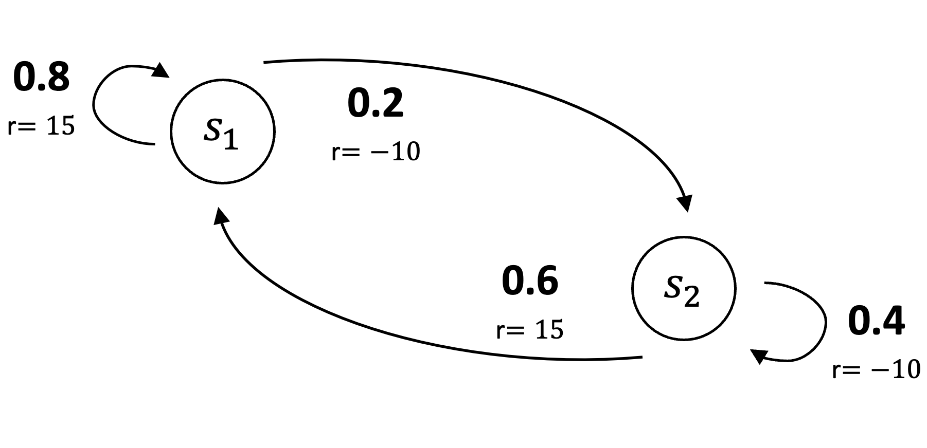 |
Using the Bellman expectation equation in matrix form (Equation \(\eqref{eq:bellman_matrix}\)), the value function can be computed as follows:
\[ \begin{equation} \nonumber \begin{bmatrix} v_{1} \\ v_{2} \end{bmatrix} = \begin{bmatrix} 10 \\ 5 \end{bmatrix} + 0.9 \begin{bmatrix} 0.8 & 0.2 \\ 0.6 & 0.4 \end{bmatrix} \begin{bmatrix} v_{1} \\ v_{2} \end{bmatrix} \end{equation} \]
\[ \begin{equation} \nonumber \begin{bmatrix} v_{1} \\ v_{2} \end{bmatrix} - \Bigg ( 0.9 \begin{bmatrix} 0.8 & 0.2 \\ 0.6 & 0.4 \end{bmatrix} \begin{bmatrix} v_{1} \\ v_{2} \end{bmatrix} \Bigg ) = \begin{bmatrix} 10 \\ 5 \end{bmatrix} \end{equation} \]
\[ \begin{equation} \nonumber \Bigg ( \begin{bmatrix} 1 & 0 \\ 0 & 1 \end{bmatrix} - 0.9 \begin{bmatrix} 0.8 & 0.2 \\ 0.6 & 0.4 \end{bmatrix} \Bigg ) \begin{bmatrix} v_{1} \\ v_{2} \end{bmatrix} = \begin{bmatrix} 10 \\ 5 \end{bmatrix} \end{equation} \]
\[ \begin{equation} \nonumber \begin{bmatrix} v_{1} \\ v_{2} \end{bmatrix} = \Bigg ( \begin{bmatrix} 1 & 0 \\ 0 & 1 \end{bmatrix} - 0.9 \begin{bmatrix} 0.8 & 0.2 \\ 0.6 & 0.4 \end{bmatrix} \Bigg )^{-1} \begin{bmatrix} 10 \\ 5 \end{bmatrix} = \begin{bmatrix} 89.02 \\ 82.93 \end{bmatrix} \end{equation} \]
Note we arbitrarily selected the discount rate \(\gamma=0.9\).
The Bellman Optimality Equations
While the Bellman expectation equations allow us to evaluate the value of a given policy, our ultimate goal is not just to assess specific policies but to identify the “best” policy. Formally, in a finite MDP — characterized by a finite number of states, actions, and rewards — a policy \(\pi\) is considered better than another policy \(\pi'\) if and only if \(V_\pi(s) \geq V_{\pi’}(s)\) for every state \(s \in \mathcal{S}\). Similarly, in terms of the action-value function, a policy is optimal if \(Q_\pi(s, a) \geq Q_{\pi’}(s, a)\) for all states \(s \in \mathcal{S}\) and all actions \(a \in \mathcal{A}\). The best or optimal policy \(\pi_*\), which guarantees expected returns at least as high as any other policy, can be found by solving the Bellman optimality equations and applying greedy action selection.
In any state \(s\), a greedy action with respect to the state-value function \(V_\pi\) is the action that maximizes the expected one-step-ahead value \(\arg\max_a \mathbb{E}[r_{t+1} + \gamma V_\pi(s_{t+1}) \mid s_t=s, a_t=a]\). It thus follows that a greedy policy with respect to \(V_\pi\) selects the maximizing action in every state. The optimal policy, then, is the greedy policy with respect to the optimal state-value function \(V_*\):
\[ \begin{equation}\nonumber V_*(s) = \max_\pi V_\pi(s) \;. \end{equation} \]
Thus, if \(V_*\) is known, selecting the greedy action in each state will result in the optimal policy. Similarly, the optimal action-value function can be used to derive the optimal policy:
\[ \begin{equation}\nonumber Q_*(s, a) = \max_\pi Q_\pi(s, a) \;. \end{equation} \]
The optimal state-value function, \(V_*\), is found by solving the state-value Bellman optimality equation:
\[ \begin{align*} V_* (s) &= \max_{a} Q_*(s,a) \\ &= \max_{a} \left( R(s,a) + \gamma \sum_{s’ \in \mathcal{S}} P(s,a,s’) V_* (s’) \right) \;. \end{align*} \]
The optimal action-value function \(Q_*\) is derived by solving the action-value Bellman optimality equation:
\[ \begin{align*} Q_* (s,a) &= R(s,a) + \gamma \sum_{s’ \in \mathcal{S}} P(s,a,s’) V_* (s’) \\ &= R(s,a) + \gamma \sum_{s’ \in \mathcal{S}} P(s,a,s’) \max_{a’} Q_* (s’, a’) \;. \end{align*} \]
Unlike the Bellman expectation equations, the Bellman optimality equations introduce the \(\max\) operator, which defines the greedy action and renders the equations non-linear. As a result, they cannot be solved directly as in Equation \(\eqref{eq:bellman_matrix}\). Nonetheless, the Bellman optimality equations are foundational in reinforcement learning. As outlined in the dynamic programming for MDPs note, there are various iterative methods for solving these equations.
Citation
Landers, Matthew. "Value Functions and Policies." mattlanders.net, June 11, 2024. mattlanders.net/value-functions-and-policies.
@article{landers2024value,
  title = {Value Functions and Policies},
  author = {Landers, Matthew},
  journal = {mattlanders.net},
  year = {2024},
  month = {June},
  url = "mattlanders.net/value-functions-and-policies"
}
References
- Markov Decision Processes, Lectures on Reinforcement Learning (2015)
David Silver
- Algorithms for Reinforcement Learning, Synthesis Lectures on Artificial Intelligence and Machine Learning (2019)
Csaba Szepesvari
- Reinforcement Learning: An Introduction (2018)
Richard S. Sutton and Andrew G. Barto
- Markov Decision Processes: Discrete Stochastic Dynamic Programming (1994)
Martin L. Puterman
- MDPs, Reinforcement Learning (2019)
Shipra Agrawal