Double Q-learning

Revised June 16, 2025

The Model Free Control and Deep Q-Learning notes are optional but recommended background reading.

The technical density of this note may suggest that Double Q-learning is algorithmically complex. In fact, it is remarkably simple. Standard Q-learning uses a single action-value function to both select and evaluate actions:

\[ \begin{align} \delta_{t} &= r_{t+1} + \gamma \max_{a’} Q(s_{t+1},a’) - Q(s_t, a_t) \label{eq:q-learning} \\ Q(s_t, a_t) &\gets Q(s_t, a_t) + \alpha \delta_{t} \;. \nonumber \end{align} \]

This, however, is prone to overestimation bias as a general statistical consequence of maximizing over random variables (i.e, due to the use of the \(\max\) operator in Equation \(\eqref{eq:q-learning}\)). The bias is not attributable to any single source of error; it can emerge from function approximation, stochastic transitions, or non-stationarity. Although uniform overestimation preserves relative action preferences and leaves the policy unaffected, in practice this bias often causes poor states to be assigned high value, leading to suboptimal updates and, under function approximation, potential divergence. More precisely, even when estimation errors are unbiased across actions, the \(\max\) operator tends to select overestimated values both in expectation and in individual samples.

Double Q-learning mitigates this bias by maintaining two independent estimators \(Q^A\) and \(Q^B\). At each update, one estimator is selected at random to determine the greedy action and is then updated using the value assigned by the other estimator. For example, if \(Q^A\) is being updated, the greedy action is selected using \(Q^A\) and evaluated using \(Q^B\):

\[ \begin{align*} \delta_t &= r_{t+1} + \gamma Q^B(s_{t+1}, \max_{a’} Q^A(s_{t+1}, a_{t+1})) - Q^A(s_t, a_t) \\ Q^A(s_t, a_t) &\gets Q^A(s_t, a_t) + \alpha \delta_t \;. \end{align*} \]

Despite its algorithmic simplicity, Double Q-learning is motivated by a nontrivial mathematical analysis.

Expected Error for Q-learning

To formally prove that Q-learning overestimates values in expectation, consider a state \(s'\) for which all true action-values are equal: \(Q^*(s’, a) = V^*(s’)\) for all \(a \in \mathcal{A}\). Let the estimated action-values be modeled as:

\[ \begin{equation}\label{eq:q-error} Q_t(s’, a) = V^*(s’) + X_a \;, \end{equation} \]

where the error terms \(X_a\) are independent and identically distributed (i.i.d.) random variables drawn from a uniform distribution \(U[-\epsilon, \epsilon]\) for some \(\epsilon > 0\). Because \(X_a \sim U[-\epsilon, \epsilon]\), each \(X_a\) has zero mean: \(\mathbb{E}[X_a] = 0\), due to the symmetry of the uniform distribution about zero. The estimator is therefore unbiased for each action, ensuring that any overestimation arises solely from the maximization step, not from systematic bias in the individual estimates.

Q-learning estimates the value of \(s'\) using \(\max_{a’} Q_t(s’, a’)\). Substituting the decomposition from Equation \(\eqref{eq:q-error}\) gives:

\[ \begin{align*} \max_{a’} Q_t(s’, a’) &= \max_{a’} \left(V^*(s’) + X_{a’}\right) \\ &= V^*(s’) + \max_{a’} X_{a’} \;, \end{align*} \]

since \(V^*(s’)\) is constant with respect to the maximization. Taking the expectations yields:

\[ \begin{align*} \mathbb{E}\left[\max_{a’} Q_t(s’, a’)\right] &= V^*(s’) + \mathbb{E}\left[\max_{a’} X_{a’}\right] \\ \mathbb{E}\left[\max_{a’} Q_t(s’, a’) - V^*(s’)\right] &= \mathbb{E}\left[\max_{a’} X_{a’}\right] \;. \end{align*} \]

Let \(Y = \max_{a’} X_{a’}\). To compute \(\mathbb{E}[Y]\), we require the probability density function (PDF) of \(Y\), since the expectation of a continuous random variable is defined as an integral over its density:

\[ \begin{equation}\label{eq:y-expectation} \mathbb{E}[Y] = \int_{-\epsilon}^{\epsilon} y \cdot f_Y(y) \, dy \;. \end{equation} \]

While the PDF can be derived directly, it is simpler in this setting to first compute the cumulative distribution function (CDF), because \(X_{a’}\) are i.i.d. and uniformly distributed on \([-\epsilon, \epsilon]\) and the maximum of i.i.d. variables reduces to a product of marginals. Formally, for \(Y = \max_{a’} X_{a’}\), the CDF is:

\[ \begin{align} F_Y(y) &= P(Y \le y) \nonumber \\ &= P(X_1 \le y, \dots, X_m \le y) \nonumber \\ &= \prod_{i=1}^m P(X_i \le y) \nonumber \\ &= \left(F_{X_a}(y)\right)^m \;, \label{eq:independent-cdf} \end{align} \]

where \(F_{X_a}\) is a marginal CDF. Since \(X_a \sim U[-\epsilon, \epsilon]\), these marginals take the standard form for a uniform distribution \(U[a, b]\):

\[ \begin{equation*} F_X(x) = \frac{x - a}{b - a} \quad \text{for } x \in [a, b] \;. \end{equation*} \]

Substituting \(a = -\epsilon\) and \(b = \epsilon\) yields:

\[ \begin{equation*} F_{X_a}(x) = \frac{x + \epsilon}{2\epsilon} \quad \text{for } x \in [-\epsilon, \epsilon] \;. \end{equation*} \]

Plugging these marginals into Equation \(\eqref{eq:independent-cdf}\) gives:

\[ \begin{equation*} F_Y(y) = \left(\frac{y + \epsilon}{2\epsilon}\right)^m \quad \text{for } y \in [-\epsilon, \epsilon] \;. \end{equation*} \]

Differentiating the CDF gives the PDF:

\[ \begin{align*} f_Y(y) &= \frac{d}{dy}F_Y(y) \\ &= \frac{d}{dy} \left(\frac{y+\epsilon}{2\epsilon}\right)^m \\ &= \frac{m}{2\epsilon} \left(\frac{y+\epsilon}{2\epsilon}\right)^{m-1} \;, \quad y \in [-\epsilon, \epsilon] \;. \end{align*} \]

Substituting into Equation \(\eqref{eq:y-expectation}\):

\[ \begin{align*} \mathbb{E}[Y] &= \int_{-\epsilon}^{\epsilon} y \cdot \frac{m}{2\epsilon} \left(\frac{y+\epsilon}{2\epsilon}\right)^{m-1} dy \;. \end{align*} \]

Let \(u = (y + \epsilon)/(2\epsilon)\) so that \(y = 2\epsilon u - \epsilon\) and \(dy = 2\epsilon \, du\), mapping \(y \in [-\epsilon, \epsilon]\) to \(u \in [0, 1]\):

\[ \begin{align*} \mathbb{E}[Y] &= \int_0^1 (2\epsilon u - \epsilon) \cdot \frac{m}{2\epsilon} u^{m-1} \cdot 2\epsilon \, du \\ &= m\epsilon \int_0^1 (2u - 1) u^{m-1} du \\ &= m\epsilon \int_0^1 (2u^m - u^{m-1}) du \\ &= m\epsilon \left( \frac{2}{m+1} - \frac{1}{m} \right) \\ &= \epsilon \cdot \frac{m-1}{m+1} \;. \end{align*} \]

Since \(m \ge 2\) and \(\epsilon > 0\),

\[ \begin{equation*} \mathbb{E}[\max_a X_a] = \epsilon \cdot \frac{m - 1}{m + 1} > 0 \;. \end{equation*} \]

Q-learning, therefore, overestimates the value of \(s'\) in expectation. The bias increases with both the number of actions \(m\) and the noise scale \(\epsilon\).

Deterministic Error for Q-learning

While maximization over random estimation errors yields overestimation in expectation, a complementary deterministic result provides a lower bound on overestimation at a fixed state, under structural constraints on the estimation errors \(X_a = Q_t(s, a) - V^*(s)\) (Equation \(\eqref{eq:q-error}\)).

Consider a state \(s\) such that all true action-values are equal:

\[ \begin{equation}\label{eq:all-true-values-equal} Q^*(s, a) = V^*(s) \quad \text{for all } a \in \mathcal{A} \;. \end{equation} \]

Assume the errors \(X_a\) satisfy two constraints. First, zero-sum bias:

\[ \begin{equation}\label{eq:zero-mean} \sum_{a=1}^m X_a = 0 \;, \end{equation} \]

and second, fixed nonzero variance:

\[ \begin{equation}\label{eq:mse} \frac{1}{m} \sum_{a=1}^m X_a^2 = C > 0 \;, \end{equation} \]

where \(m = |\mathcal{A}|\). (Note that these jointly imply \(m \ge 2\): if \(m = 1\), then Equation \(\eqref{eq:zero-mean}\) forces \(X_1 = 0\), contradicting Equation \(\eqref{eq:mse}\)).

We now determine the minimum possible value of the algebraically maximal error (i.e.; the largest signed error, as opposed to the largest absolute error), \(\max_a X_a\), subject to constraints \(\eqref{eq:zero-mean}\) and \(\eqref{eq:mse}\).

To obtain this tight lower bound, consider the configuration in which \(m - 1\) actions have error \(x > 0\), and the remaining action offsets their sum:

\[ \begin{equation}\label{eq:errors} X_1 = \dots = X_{m - 1} = x \;, \quad X_m = -(m - 1)x \;. \end{equation} \]

This configuration is known to minimize the algebraic maximum error, \(x = \max_a X_a\), under constraints \(\eqref{eq:zero-mean}\) and \(\eqref{eq:mse}\), though we do not prove this here as the result is standard in convex optimization and information theory. We simply verify that the configuration satisfies the constraints and then solve for \(x\) to obtain the bound.

The zero-mean constraint is satisfied:

\[ \begin{equation*} \sum_{a=1}^m X_a = (m - 1)x + ( - (m - 1)x ) = 0 \;. \end{equation*} \]

To verify the variance constraint, compute the sum of squared errors:

\[ \begin{align*} \sum_{a=1}^m X_a^2 &= (m - 1)x^2 + (-(m - 1)x)^2 \\ &= (m - 1)x^2 + (m - 1)^2 x^2 \\ &= x^2 (m - 1)(1 + m - 1) \\ &= x^2 m(m - 1) \;. \end{align*} \]

Dividing by \(m\) gives the mean squared error:

\[ \begin{equation*} \frac{1}{m} \sum_{a=1}^m X_a^2 = x^2 (m - 1) \;. \end{equation*} \]

Imposing the constraint \(x^2 (m - 1) = C\) (Equation \(\eqref{eq:mse}\)) gives:

\[ \begin{align*} x^2 (m - 1) &= C \\ x^2 &= \frac{C}{m - 1} \\ x &= \sqrt{\frac{C}{m - 1}} \;. \end{align*} \]

Of the \(m\) errors, \(m - 1\) are equal to \(x\) and one equals \(-(m - 1)x\) (by Equation \(\eqref{eq:errors}\)). Because \(x > 0\) (given \(C > 0\) and \(m \ge 2\)) and \(-(m-1)x\) is non-positive, the algebraically largest error is:

\[ \begin{equation}\label{eq:main-bound} \max_a X_a = x = \sqrt{\frac{C}{m - 1}} \;. \end{equation} \]

Given that the configuration in Equation \(\eqref{eq:errors}\) minimizes the algebraically maximal error under the constraints, this establishes a lower bound on worst-case overestimation. Specifically, any configuration satisfying constraints \(\eqref{eq:zero-mean}\) and \(\eqref{eq:mse}\) must exhibit an overestimation of at least \(\sqrt{C/(m - 1)}\) in individual samples.

Double Q-learning

Double Q-learning mitigates overestimation bias by decoupling action selection from evaluation. It maintains two independent value estimators, \(Q^A\) and \(Q^B\). At each step, one of the two estimators, typically chosen at random, is updated. The target is computed by selecting the greedy action under the estimator being updated and using the other estimator to assign a value to that action. For example, if \(Q^A\) is being updated, the greedy action is selected using \(Q^A\) and evaluated using \(Q^B\):

\[ \begin{align*} \delta_t &= r_{t+1} + \gamma Q^B(s_{t+1}, \max_{a’} Q^A(s_{t+1}, a’)) - Q^A(s_t, a_t) \\ Q^A(s_t, a_t) &\gets Q^A(s_t, a_t) + \alpha \delta_t \;. \end{align*} \]

Expected Error for Double Q-learning

Without loss of generality, let the action be selected by \(Q^A\) and its value evaluated by \(Q^B\). Assume further that all action-values equal the true state value \(Q^*(s,a) = V^*(s)\) for all \(a\), as in Equation \(\eqref{eq:all-true-values-equal}\). Define the estimation error at state \(s\) as

\[ \begin{equation*} Y_a = Q^B(s, a) - V^*(s) \;, \end{equation*} \]

where \(V^*(s)\) is the true state value. Suppose the errors \(Y_a\) are zero-mean across runs (i.e., \(\mathbb{E}[Y_a] = 0\) for all \(a\)) and statistically independent of the action \(a^*\) selected by \(Q^A\). Then the expected error in the Double Q-learning estimate satisfies:

\[ \begin{equation*} \mathbb{E}[Q^B(s, a^*) - V^*(s)] = \mathbb{E}[Y_{a^*}] = 0 \;. \end{equation*} \]

Thus, there exists a set of conditions under which Double Q-learning eliminates the overestimation bias of standard Q-learning in expectation.

Deterministic Error for Double Q-learning

Unlike Q-learning, Double Q-learning can, under structural constraints, produce exact value estimates in individual states. We analyze this deterministic behavior by imposing the same conditions used in the Q-learning case. Specifically, applying the same zero-mean and fixed-variance constraints (Equations \(\eqref{eq:zero-mean}\) and \(\eqref{eq:mse}\)), choose the extremal pattern from Equation \(\eqref{eq:errors}\):

\[ \begin{align*} X_1=\dots=X_{m-1}=x,\qquad X_m=-(m-1)x,\qquad x= \sqrt{\frac{C}{m-1}} \;. \end{align*} \]

As established in the previous section, this configuration ensures that any of the first \(m - 1\) actions attains the maximum of \(Q^A\). Without loss of generality, let the greedy action be denoted by \(a^* = a_1\). The Double Q-learning estimate is then:

\[ \begin{equation*} Q_B(s, a_1) = V^*(s) + Y_{a_1} \;. \end{equation*} \]

Zero error in this estimate requires:

\[ \begin{equation*} Y_{a_1} = 0 \;. \end{equation*} \]

Under the constraints of Equations \(\eqref{eq:zero-mean}\) and \(\eqref{eq:mse}\), the following assignment is admissible:

\[ \begin{equation}\label{eq:dq-assignment} Y_{a_1} = 0 \;, \quad Y_2 = \sqrt{\frac{mC}{2}} \;, \quad Y_3 = -\sqrt{\frac{mC}{2}} \;, \quad Y_i = 0 \quad \text{for } i = 4, \dots, m \;. \end{equation} \]

This configuration satisfies the zero-mean constraint (Equation \(\eqref{eq:zero-mean}\)):

\[ \begin{align*} \sum_a Y_a &= Y_{a_1} + Y_2 + Y_3 + \sum_{i=4}^m Y_i \\ &= 0 + \sqrt{\frac{mC}{2}} - \sqrt{\frac{mC}{2}} + 0 \\ &= 0 \;. \end{align*} \]

The total squared error is:

\[ \begin{align*} \sum_a Y_a^2 &= Y_{a_1}^2 + Y_2^2 + Y_3^2 + \sum_{i=4}^m Y_i^2 \\ &= 0 + \frac{mC}{2} + \frac{mC}{2} + 0 \\ &= mC \;, \end{align*} \]

which yields a mean-squared error of:

\[ \begin{equation*} \frac{1}{m} \sum_a Y_a^2 = C \;, \end{equation*} \]

satisfying the variance constraint (Equation \(\eqref{eq:mse}\)).

This construction results in:

\[ \begin{align*} |Q_B(s, a^*) - V^*(s)| = |Y_{a_1}| = 0 && \text{by Equation } \eqref{eq:dq-assignment} \;. \end{align*} \]

Thus, for \(m \ge 3\), the absolute error in the Double Q-learning estimate can be zero, even under the same constraints that impose a nonzero deterministic lower bound for Q-learning. In particular, Q-learning guarantees

\[ \begin{align*} \max_a X_a \ge \sqrt{\frac{C}{m - 1}} && \text{cf. Equation } \eqref{eq:main-bound} \;, \end{align*} \]

while Double Q-learning allows

\[ \begin{equation*} |Y_{a^*}| = 0 \;. \end{equation*} \]

Double Q-learning thus eliminates not only the expected overestimation bias, but also the deterministic lower bound on absolute error when \(m \ge 3\).

Deterministic error for Double Q-learning when \(m = 2\)

Although unrealistic in practice, the case \(m = 2\) serves as a degenerate boundary condition that must be treated separately. With only two actions, the zero-mean and fixed-variance constraints leave no flexibility: the error structure is fully determined. Unlike the \(m \ge 3\) case, where the constraints admit many configurations (including some with zero absolute error), here Equation \(\eqref{eq:zero-mean}\) forces \(X_2 = -X_1\).

Substituting this identity into the mean-squared error expression gives

\[ \begin{align*} \frac{1}{2}(X_1^2 + X_2^2) &= \frac{1}{2}(X_1^2 + (-X_1)^2) \\ &= \frac{1}{2}(2 X_1^2) \\ &= X_1^2 \\ &= C \;. \end{align*} \]

Thus, \(X_1 = \pm \sqrt{C}\) and \(X_2 = \mp \sqrt{C}\). The valid error pairs are therefore \((\sqrt{C}, -\sqrt{C})\) or \((-\sqrt{C}, \sqrt{C})\). Since the selected action \(a^*\) maximizes \(Q^A(s, a) = V^*(s) + X_a\) and \(C > 0\), the maximizer is always the action with error \(+\sqrt{C}\). Therefore,

\[ \begin{equation*} X_{a^*} = \sqrt{C} \end{equation*} \]

in all cases.

The \(Y_a\) errors are subject to the same constraints. By identical reasoning, the only valid configurations are \((\sqrt{C}, -\sqrt{C})\) and \((-\sqrt{C}, \sqrt{C})\).

Since \(a^*\) is determined by the \(X_a\) values and the \(Y_a\) configuration is independent, \(Y_{a^*}\) may take either value in the pair. In both cases, the absolute error is

\[ \begin{equation*} |Y_{a^*}| = \sqrt{C} \;. \end{equation*} \]

Thus, for \(m = 2\), the Double Q-learning estimate incurs deterministic absolute error \(\sqrt{C}\).

Double DQN

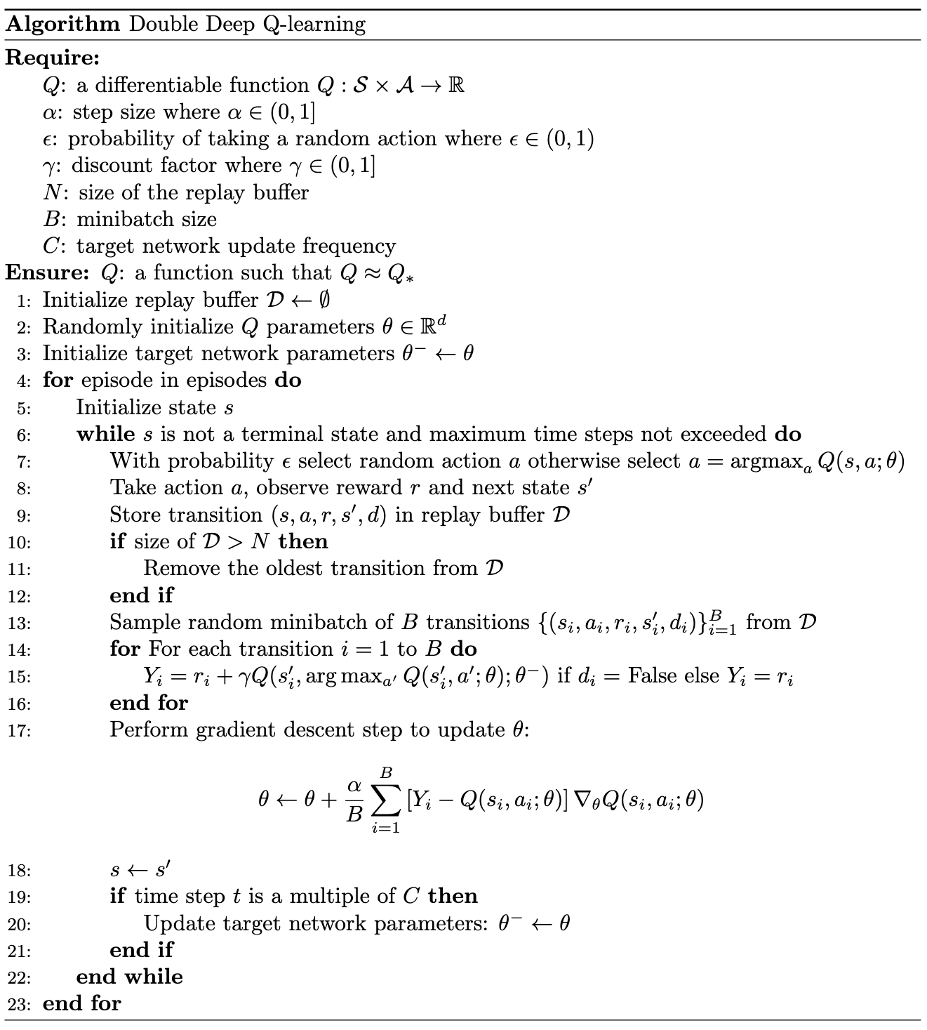
It is natural to assume that Double Deep Q-learning, the deep variant of Double Q-learning, would require two fully decoupled networks. In practice, however, it repurposes the DQN's target network to serve as the second value function. That is, the algorithm is identical to DQN except for the update target, which becomes:

\[ \begin{equation*} Y_t^{DDQN} = r + \gamma Q(s’, \max_{a’} Q(s’, a’; \theta); \theta^-) \;. \end{equation*} \]

As in a standard DQN, the target network is updated by periodic copying from the online network.

References

Double Q-learning, Advances in neural information processing systems (2010)

Hado van Hasselt

Deep Reinforcement Learning with Double Q-learning, Proceedings of the AAAI conference on artificial intelligence (2016)

Hado van Hasselt, Arthur Guez, and David Silver

Addressing Function Approximation Error in Actor-Critic Methods, International conference on machine learning (2018)

Scott Fujimoto, Herke van Hoof, and David Meger