Model-Free Prediction

Revised October 19, 2024

The Dynamic Programming for Solving MDPs note is optional but recommended background reading.

Both Value Iteration and Policy Iteration are considered “exact” methods because they are guaranteed to converge to the optimal value function \(V_*\) in the limit. Determining the optimal value function exactly offers clear advantages; however, these methods require a perfect model of the environment's transition probabilities and rewards, which are often unavailable in practice. Model-free methods relax the assumption of full access to the environment's dynamics. Instead, they estimate the optimal value function underlying an MDP through stochastic approximation. Before discussing methods for estimating the optimal value function, it is useful to first explore approaches for estimating an arbitrary value function \(V_\pi\). We refer to this as the prediction or policy evaluation problem.

Monte Carlo Methods

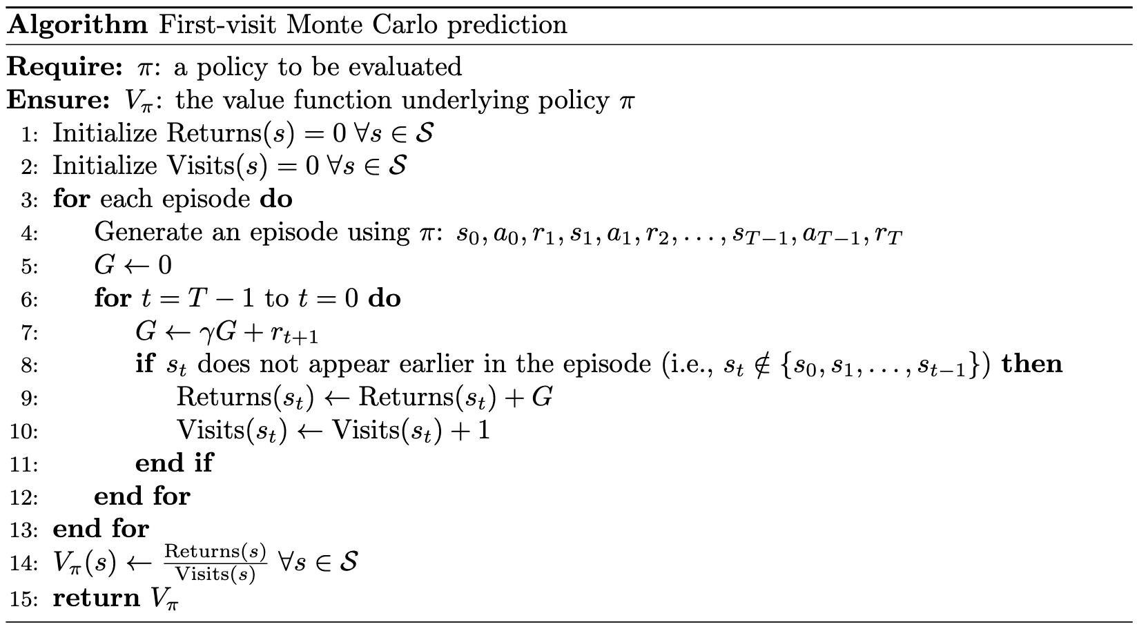
Monte Carlo (MC) methods estimate the value of a state \(s\) under a policy \(\pi\) by averaging the returns observed from starting in \(s\) across multiple independent episodes. In First-visit MC, the value function \(V_\pi(s)\) is estimated by averaging the returns obtained after the first visit to \(s\) in each episode.

Every-visit MC, by contrast, averages the returns earned after all visits to \(s\) within each episode.

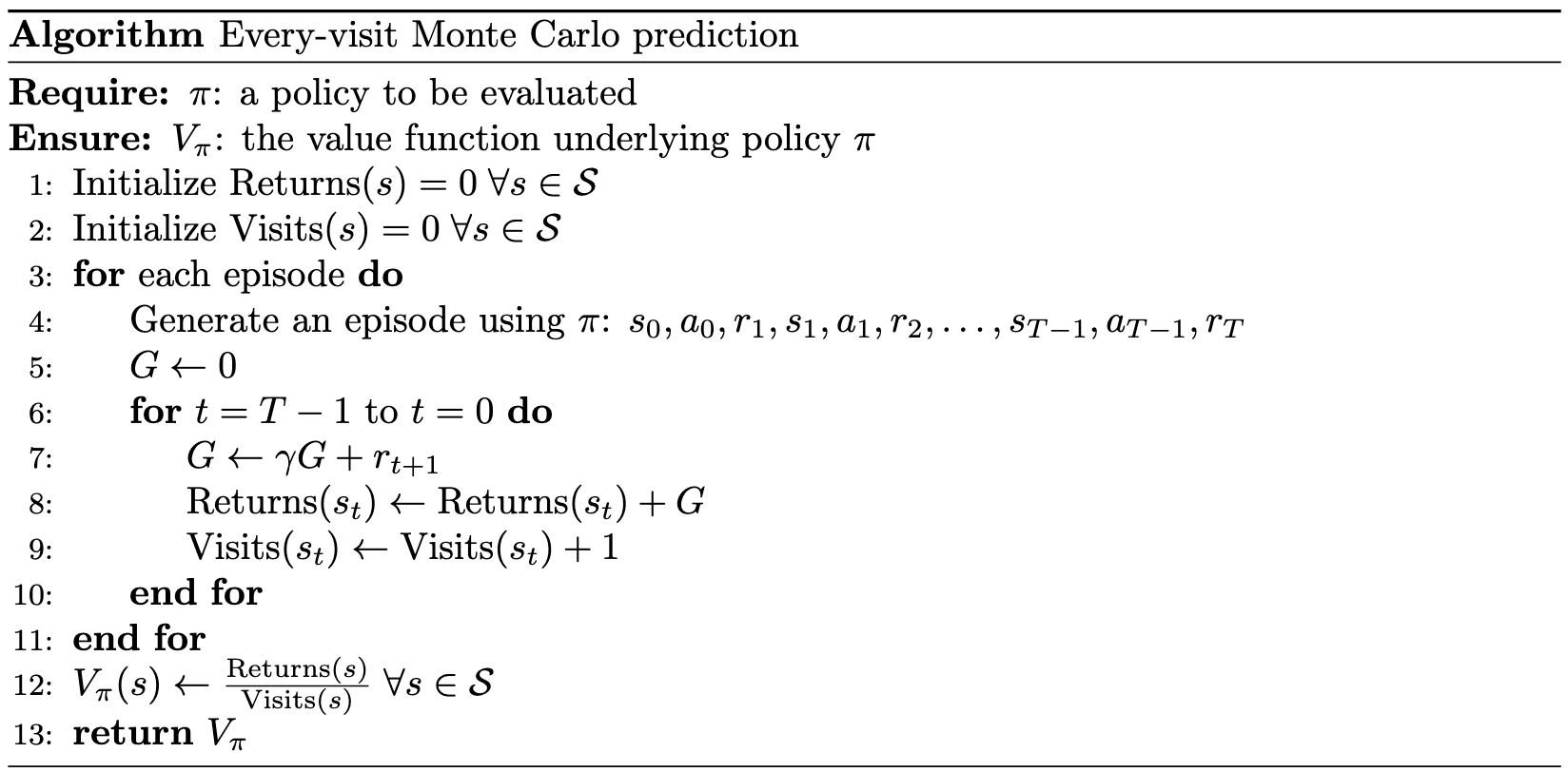Recall that the agent's performance is measured by total discounted return: \(G_t = r_{t+1} + \gamma r_{t+2} + \cdots + \gamma^{T-t-1} r_T\). In both first-visit and every-visit MC methods, the return calculation begins at the penultimate state \(s_{T-1}\), where \(G = r_T\). For \(t = T-2\), the return becomes \(G = r_{T-1} + \gamma r_T\). At \(t = T-3\), the return is \(G = r_{T-2} + \gamma r_{T-1} + \gamma^2 r_T\). This process continues backward until \(t = 0\).

After generating one or more episodes, MC methods estimate the value of a state \(s\) by computing the sample average of the returns observed for that state. This is typically implemented by summing all returns for a state and dividing by the number of times the state was visited (see line 15 in the first-visit pseudocode and line 13 in the every-visit pseudocode). In first-visit MC, each return is an independent and identically distributed (i.i.d.) estimate of \(V_\pi(s)\) with finite variance. By the law of large numbers, the sequence of sample averages converges to the expected value \(V_\pi(s)\). Although the analysis is more complex for every-visit MC, it also converges to \(V_\pi(s)\) in the limit.

Temporal Difference Learning

While MC methods are simple, they have notable limitations. For example, their returns can exhibit high variance, they are restricted to episodic MDPs (i.e., those that terminate), and the return for a state is not known until the episode terminates. Temporal difference (TD) learning addresses these shortcomings.

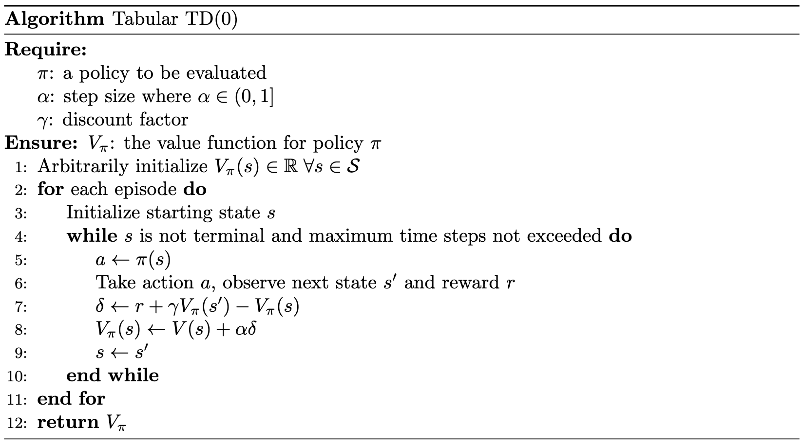
Like MC, TD methods are model-free, meaning they do not require knowledge of the environment's dynamics. However, similar to dynamic programming (DP), TD methods use bootstrapping, allowing them to update the value function before an episode ends. TD methods update a state's value using the estimated values of subsequent states. The simplest TD method, TD(0), updates the value of \(s_t\) immediately after the transition to \(s_{t+1}\) and receiving the reward \(r_{t+1}\):

\[ \begin{align} \delta_t = r_{t+1} + \gamma V(s_{t+1}) - V(s_t) \label{eq:td_error} \\ V(s_t) \gets V(s_t) + \alpha \delta_t \label{eq:td_value_update} \end{align} \]

where \(\alpha \in (0,1]\) is the learning rate.

Expanding \(\delta_t\) in Equation \(\eqref{eq:td_value_update}\), we obtain:

\[ \begin{equation}\label{eq:expanded_td_value_update} V(s_t) \gets V(s_t) + \alpha \big( r_{t+1} + \gamma V(s_{t+1}) - V(s_t) \big) \;. \end{equation} \]

In this way, TD and MC methods fundamentally differ in how the update target is defined. For an incremental update of the form:

\[ \begin{equation*} V(s_t) \gets V(s_t) + \alpha \, (\text{Target} - V(s_t)) \;, \end{equation*} \]

the MC target is the full sampled return \(G_t = r_{t+1} + \gamma r_{t+2} + \dots + \gamma^{T-t-1} r_T\), whereas the TD target is the one-step bootstrapped estimate \(r_{t+1} + \gamma V(s_{t+1})\). In the TD update, the estimated value \(V(s_{t+1})\) serves as a proxy for the entire sequence of future returns (\(\gamma r_{t+2} + \gamma^2 r_{t+3} + \dots\)) that MC methods observe only at the end of an episode. The step size parameter \(\alpha\) controls how much the observed transition updates the current estimate, balancing past information with new data.

With each iteration, the estimate of \(V(s_t)\) improves. In Equation \(\eqref{eq:td_error}\), \(\delta_t\) captures this improvement, quantifying the difference between the current estimate of \(V(s_t)\) and the updated estimate, \(r_{t+1} + \gamma V(s_{t+1})\). This difference, fundamentally an error in the current estimate, is known as the TD error.

TD learning is guaranteed to converge to \(V_\pi\) as the number of episodes \(K\) approaches infinity. For a finite number of episodes, TD(0) converges to the solution of the maximum likelihood MDP. Intuitively, TD(0) constructs an MDP, \(\hat{\mathcal{M}} = \langle \mathcal{S}, \mathcal{A}, \hat{P}, \hat{R}, \gamma \rangle\), that best fits the observed data. The dynamics for \(\hat{\mathcal{M}}\) are estimated by counting state transitions:

\[ \begin{align*} \hat{P}(s,a,s^\prime) = \frac{1}{N(s,a)} \sum_{k=1}^{K} \sum_{t=1}^{T_k} \mathbf{1}_{\{s_t^k = s, a_t^k = a, s_{t+1}^k = s^\prime\}} && \hat{R}(s,a) = \frac{1}{N(s,a)} \sum_{k=1}^{K} \sum_{t=1}^{T_k} r_{t+1}^k \mathbf{1}_{\{s_t^k = s, a_t^k = a\}} \;, \end{align*} \]

where \(N(s,a)\) is the total number of times action \(a\) is taken in state \(s\) across all \(K\) episodes, and \(\mathbf{1}_{x}\) is the indicator function, which equals 1 if the condition \(x\) holds and 0 otherwise.

\(n\)-step TD methods

Although TD methods address certain limitations of MC, they introduce bias through bootstrapping, as they depend on initial estimates of \(V(s)\) or \(Q(s, a)\) for all states \(s\) and state-action pairs \((s, a)\), respectively. These assumptions affect subsequent value updates as can be seen in \(\eqref{eq:td_error}\). MC methods, by contrast, are unbiased, as they do not depend on initial value estimates.

Given the complementary advantages of MC and TD, it is natural to consider methods that integrate both. \(n\)-step TD methods provide such a framework, offering a flexible trade-off between MC and TD(0). These methods can be viewed as existing along a continuum, with MC at one end and TD(0) at the other.

Recall that MC methods update the target \(V\) after the full trajectory has been observed, while TD(0) updates the target after observing only the next reward (see Equation \(\eqref{eq:td_value_update}\)). As the name suggests, \(n\)-step methods update the target after observing \(n\) steps. For example, the one-step return updates the target based on the first reward and the estimated discounted value of the next state:

\[ \begin{equation}\label{eq:one-step-td} G_{t:t+1} = r_{t+1} + \gamma V_t(s_{t+1}) \;, \end{equation} \]

where \(V_t: \mathcal{S} \rightarrow \mathbb{R}\) is the estimate of \(V_\pi\) at time \(t\), and \(G_{t:t+1}\) is the truncated return from time \(t\) to \(t+1\). Notice that Equation \(\eqref{eq:one-step-td}\) is the TD(0) update, corresponding to the TD error term in \(\eqref{eq:expanded_td_value_update}\).

We can similarly define the two-step return as:

\[ \begin{equation*} G_{t:t+2} = r_{t+1} + \gamma r_{t+2} + \gamma^2 V_{t+1}(s_{t+2}) \;, \end{equation*} \]

and the general \(n\)-step return as:

\[ \begin{equation}\label{eq:n-step_return} G_{t:t+n} = r_{t+1} + \gamma r_{t+2} + \dots + \gamma^{n-1} r_{t+n} + \gamma^n V_{t+n-1}(s_{t+n}) \;, \end{equation} \]

where \(\gamma^n V_{t+n-1}(s_{t+n})\) represents the estimate of the future returns beyond step \(n\), replacing the unknown returns \(\gamma^n r_{t+n+1} + \gamma^{n+1} r_{t+n+2} + \dots + \gamma^{T-t-1} r_{T}\), as described for TD(0).

Our value function can then be defined as:

\[ \begin{align*} V_{t+n}(s_t) = V_{t+n-1}(s_t) + \alpha \left( G_{t:t+n} - V_{t+n-1}(s_t) \right) && \text{cf. }\eqref{eq:expanded_td_value_update} \;, \end{align*} \]

There is a practical concern we must address when \(n > 1\); to calculate \(\eqref{eq:n-step_return}\) we must know future rewards. That is, when we transition from \(t\) to \(t+1\) our computation requires \(r_{t+1}, r_{t+2}, \dots, r_{t+n}\), however only \(r_{t+1}\) is available at \(t+1\). This means to compute \(\eqref{eq:n-step_return}\) we have to wait until transition \(t+n\). We can account for this as illustrated in the pseudocode below.

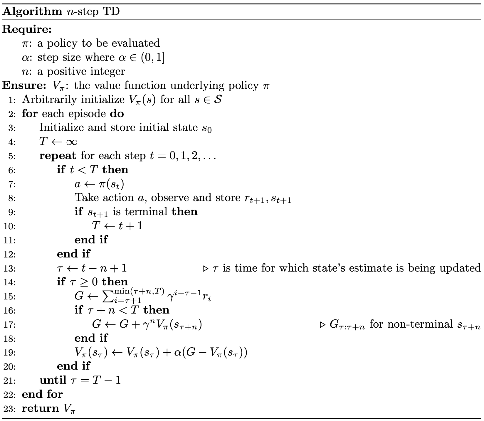No updates are made for the first \(n-1\) steps of each episode, as not enough rewards have been observed to compute the expected return \(G\). To compensate, the algorithm performs \(n-1\) updates after the episode terminates at time \(T\). For example, suppose \(n=3\) and \(s_5\) is a terminal state. When \(t=0\), updating \(V(s_0)\) requires \(r_1\), \(r_2\), and \(r_3\). However, \(\tau = 0 - 3 + 1 = -2 < 0\), meaning there is not yet enough information to update \(V(s_0)\); we are still two steps away from having enough information to calculate \(G_0\). In this example, an update is first performed when \(\tau = t-n+1 = 0\), i.e., when \(t=2\). At this point, the return \(G\) is computed as \(G = r_1 + \gamma r_2 + \gamma^2 r_3\) according to the definition on line 15. The first time \(T \neq \infty\) occurs at \(t=4\) (since \(s_5\) is terminal), at which point we set \(T = 5\). The update loop continues until \(\tau = T-1\). In our example where the episode terminates at \(T=5\), the final update is performed when \(\tau\) reaches 4. This update is for the penultimate state, \(s_4\), using the final reward \(r_5\). The value of the terminal state \(s_5\) is not updated, as its value is defined as 0. Finally, the summation on line 15 includes a \(\min\) operator to ensure that the upper limit does not exceed the end of the episode. Without it, the sum would always extend to \(\tau+n\). For instance, in the update for \(s_4\) with \(\tau=4\) and \(T=5\), if \(n=3\) the upper limit would be \(\tau+n=7\), and the formula would incorrectly try to access rewards \(r_6\) and \(r_7\), which do not exist. Using \(\min(\tau+n,T)\) sets the upper limit to \(\min(7,5)=5\), so the summation includes only \(i=5\) and yields the correct return \(G=r_5\).

TD(\(\lambda\))

While estimating returns using a single \(n\) is reasonable, averaging over multiple \(n\) values is often more effective. TD(\(\lambda\)) uses eligibility traces to define mixing coefficients for multi-step returns. Specifically, an eligibility trace parameter \(\lambda \in [0,1]\) interpolates between TD(0) and MC methods:

\[ \begin{equation}\label{eq:td-lambda} G^\lambda_t = (1-\lambda) \sum_{n=1}^\infty \lambda^{n-1} G^{(n)}_{t:t+n} \;, \end{equation} \]

where \((1-\lambda)\) is a normalization factor ensuring the weights \(\lambda^{n-1}\) sum to 1.

In TD(\(\lambda\)), the one-step return receives the largest weight, \((1-\lambda)\), with each subsequent \(n\)-step return receiving progressively smaller weights: \((1-\lambda)\lambda\) for two steps, \((1-\lambda)\lambda^2\) for three steps, and so on.

Once an \(n\)-step return includes a terminal state, all subsequent \(n\)-step returns (i.e., those for larger values of \(n\)) converge to the conventional return from the initial state \(t\) to the terminal state \(T\). To differentiate between \(n\)-step returns that exclude a terminal state and those that include one, Equation \(\eqref{eq:td-lambda}\) can be reformulated as follows:

\[ \begin{align}\label{eq:multistep_predictions} G^\lambda_t = (1-\lambda) \sum_{n=1}^{T-t-1} \lambda^{n-1} G^{(n)}_{t:t+n} + \color{red}{\lambda^{T-t-1} G_t} \;, \end{align} \]

where the red term, \(\lambda^{T-t-1} G_t\), is the conventional return weighted by \(\lambda^{T-t-1}\).

For example, if \(t=2\) and \(T=6\) (i.e., \(s_6\) is terminal), the equation for \(G^\lambda_t\) simplifies as follows:

\[ \begin{align*} G^\lambda_t &= (1-\lambda) \left( G^{(1)}_{2:3} + \lambda G^{(2)}_{2:4} + \lambda^2 G^{(3)}_{2:5} \right) + \lambda^3 G_2 \\ G^\lambda_t &= (1-\lambda) \left( G^{(1)}_{2:3} + \lambda G^{(2)}_{2:4} + \lambda^2 G^{(3)}_{2:5} \right) + \lambda^3 \sum_{k=0}^3 \gamma^k r_{2+k+1} \;, \end{align*} \]

This formulation illustrates why the summation in Equation \(\eqref{eq:multistep_predictions}\) terminates at \(n = T-t-1\). Consider \(G^{(4)}_{2:6}\) which, according to Equation \(\eqref{eq:n-step_return}\), expands to:

\[ \begin{equation*} G_{2:6} = r_3 + \gamma r_4 + \gamma^2 r_5 + \gamma^3 r_6 + \gamma^4 V_5(s_6) \;. \end{equation*} \]

Here, \(V_5(s_6)\) evaluates to zero because the value function at a terminal state is zero, reflecting the absence of future rewards beyond this point. For \(t+n\) values greater than six (e.g., \(G_{2:7}\)), terms such as \(r_7\) and \(V(s_7)\) would emerge, which are conceptually and practically irrelevant since they extend beyond the episode's end. This necessitates the separation and distinct handling of cases where \(n \leq T-t-1\) and \(n > T-t-1\).

Handling the terms where \(n \leq T-t-1\) and \(n > T-t-1\) separately also allows TD(\(\lambda\)) to induce MC behavior by setting \(\lambda = 1\). Under this condition, the weighted sum of \(n\)-step returns becomes zero due to the \((1-\lambda)\) term, simplifying the overall update to \(G_t\). This corresponds to a pure Monte Carlo approach, relying exclusively on the complete return. Conversely, setting \(\lambda = 0\) emphasizes the immediate one-step return, \(G^{(1)}_t\), aligning with the behavior of TD(0) — hence the name TD(0).

The value of a state can then be updated as:

\[ \begin{equation*} V_t(s_t) = V_t(s_t) + \alpha \big( G^\lambda_t - V_t(s_t) \big) \;. \end{equation*} \]

This method is known as the forward view of TD(\(\lambda\)) because the update for \(V(s_t)\) depends on the entire sequence of future rewards and states within the episode. Consequently, the update for a given state \(s_t\) can only be performed after the episode has concluded and the full lambda-return \(G^\lambda_t\) is known.

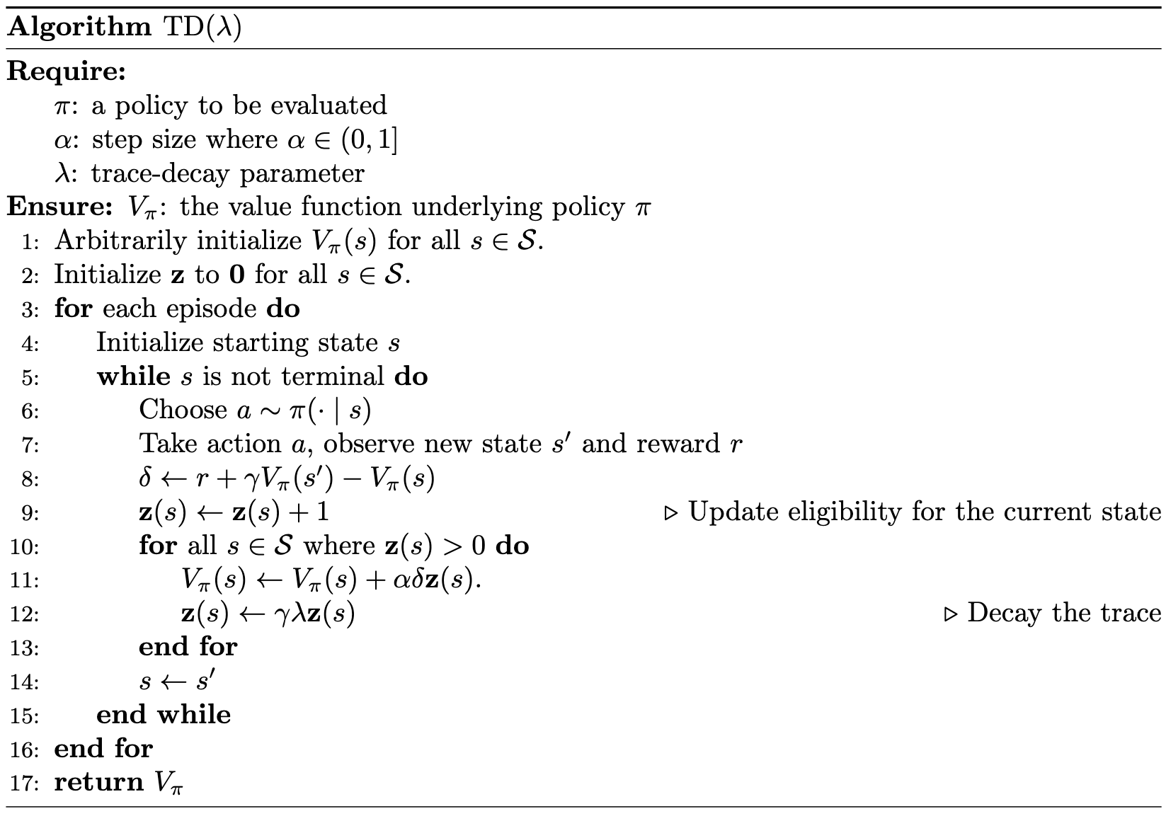
The forward view is acausal, as it relies on information about future outcomes that are not yet known at the time of the update. This characteristic highlights a practical limitation, as it presupposes knowledge of all subsequent rewards, which is not typically available in real-time decision-making scenarios. This motivates the backward view of TD(\(\lambda\)). In this approach, an eligibility trace serves as a mechanism for credit assignment, quantifying the influence of each state on future outcomes. The eligibility trace, represented by a vector \(\mathbf{z} \in \mathbb{R}^\mathcal{S}\), incorporates two heuristics: frequency and recency of state visits.

At each time step, the eligibility trace for the current state \(s = s_t\) is incremented by one, while the trace for all other states decays according to the trace-decay parameter \(\lambda \in [0,1]\):

\[ \begin{equation}\label{eq:trace-update} \textbf{z}_t(s) = \begin{cases} \gamma \lambda \textbf{z}_{t-1}(s) + 1 & \text{if } s = s_t \\ \gamma \lambda \textbf{z}_{t-1}(s) & \text{if } s \neq s_t \;. \end{cases} \end{equation} \]

When a TD error \(\delta_t\) (Equation \(\eqref{eq:td_error}\)) occurs, the value function is updated proportionally to the eligibility trace:

\[ \begin{align*} \delta_{t} &= r_{t+1} + \gamma V(s_{t+1}) - V(s_t) \;, \nonumber \\ V(s) &\gets V(s) + \alpha \delta_{t} \textbf{z}_t(s), && \forall s \in \mathcal{S}. \label{eq:backward-update} \end{align*} \]

Eligibility traces in \(\textbf{z}\) represent the extent to which each state is “eligible” for a learning update following a “reinforcing event”, defined here as the one-step TD error. When \(\lambda < 1\), earlier states are given progressively less credit for the TD error, as the trace decays. When \(\lambda = 1\), all previous states receive equal credit, and the credit diminishes only by the discount factor \(\gamma\), akin to the MC updates. Conversely, when \(\lambda = 0\), all eligibility traces are zero except for the current state \(s_t\) (cf. Equation \(\eqref{eq:trace-update}\)), reducing the update to TD(0).

Unlike the forward view, the backward view of TD(\(\lambda\)) is both incremental and causal, making it more practical for real-time applications. Crucially, this approach allows us to approximate the theoretically optimal forward view in online scenarios and to replicate it exactly in offline contexts.

Eligibility traces, while computationally more demanding than one-step methods, facilitate faster learning, particularly in environments with long-delayed rewards. This makes eligibility traces well-suited for online learning, where learning happens as the agent interacts with the environment. However, in offline settings where data can often be generated through simulations, the benefits of faster learning may not always justify the higher computational costs.

References

Model-Free Prediction, Lectures on Reinforcement Learning (2015)

David Silver

Reinforcement Learning: An Introduction (2018)

Richard S. Sutton and Andrew G. Barto

Algorithms for Reinforcement Learning, Synthesis Lectures on Artificial Intelligence and Machine Learning (2019)

Csaba Szepesvari

Reinforcement Learning: An Introduction (1998)

Richard S. Sutton and Andrew G. Barto

Learning Rates for Q-learning, Journal of Machine Learning Research (2003)

Eyal Even-Dar and Yishay Mansour