Policy Gradients

RL methods can be broadly divided into two classes: action-value methods and policy gradient methods. Action-value methods — which underlie classical algorithms such as Q-learning and its derivatives like deep Q-learning — select actions by estimating the expected return for each action in a given state. Policy gradient methods, by contrast, do not reference a value function for action selection. Instead, they directly optimize a parameterized policy \(\pi(s, a; \theta)\).

More specifically, policy gradient methods learn the parameters \(\theta\) that maximize a policy objective function \(J(\theta)\). For episodic MDPs with a deterministic initial state \(s_0\), the value function provides a natural objective: \(J(\theta) = V^{\pi_\theta}(s_0)\). For continuing MDPs, the average reward per time step serves as an alternative objective; we will explore this distinction later in this note. While this choice of objective might appear to conflict with the fundamental property of policy gradient methods — selecting actions without referencing a value function — it is consistent with this principle as the value function is used solely to guide optimization, not for action selection.

To optimize \(\theta\), policy gradient algorithms seek a local maximum of \(J(\theta)\) by ascending its gradient with respect to \(\theta\):

\[ \begin{equation}\label{eq:pg_grad} \theta_{t+1} = \theta_t + \alpha \nabla_\theta J(\theta) \;, \end{equation} \]

where \(\alpha\) is a step-size parameter and \(\nabla_\theta J(\theta) \in \mathbb{R}^d\) is a column vector of partial derivatives:

\[ \begin{equation*} \nabla_\theta J(\theta) = \left[ \frac{\partial J(\theta)}{\partial \theta_1}, \frac{\partial J(\theta)}{\partial \theta_2}, \dots, \frac{\partial J(\theta)}{\partial \theta_d} \right]^\top \;. \end{equation*} \]

When the action space is discrete and small, parameterized preferences, \(\phi(s, a; \theta)\), can be defined for each state–action pair. These preferences allow for the use of a softmax action selection strategy, an alternative to the \(\epsilon\)-greedy method. In this approach, the probability of selecting an action is proportional to the exponentiated value of its preference:

\[ \begin{equation}\label{softmax} \pi(a \mid s; \theta) \propto e^{\phi(s, a; \theta)} = \frac{e^{\phi(s, a; \theta)}}{\sum_b e^{\phi(s, b; \theta)}} \;, \end{equation} \]

Action preferences can be determined in various ways. For instance, we can use a linear combination of features, where the preferences are given by \(\phi(s, a; \theta) = \theta^\top \phi(s, a)\). Alternatively, more complex models, such as neural networks, can be used. In such cases, \(\theta\) represents the network's weights and biases.

Policy gradient methods provide distinct advantages relative to action-value methods. Action-value methods typically define policies through greedy action selection, \(\arg \max_a Q(s, a)\). This formulation imposes two fundamental constraints: computational infeasibility for large or continuous action spaces, and an inability to represent stochastic optimal policies.

While action-value methods rely on deterministic action selection, a policy admits a more general formulation as a conditional probability distribution over actions given states. For example, in continuous action spaces, instead of relying on the softmax parameterization in Equation \(\eqref{softmax}\), a policy can be represented as a Gaussian distribution for which the mean and standard deviation are computed by a neural network.

By leveraging this broader definition, policy gradient methods enable the learning of stochastic optimal policies and provide stronger convergence guarantees than action-value methods. These improved guarantees arise, in part, from the smooth change in action probabilities as a function of the learned parameters \(\theta\), as illustrated in Equation \(\eqref{softmax}\). This smoothness means the policy gradient is well-defined everywhere and varies continuously. In contrast, \(\epsilon\)-greedy action selection can produce discontinuous shifts in action probabilities: an infinitesimal change in action values may cause a different action to become optimal, resulting in an abrupt redistribution of probabilities. Such discontinuities create regions where gradients are undefined or exhibit sharp changes, which can destabilize the learning process and hinder convergence.

The Policy Gradient Theorem

Establishing theoretical guarantees for policy gradient methods requires accounting for the dependence of the value function (i.e., the function we are attempting to maximize):

\[ \begin{equation*} V_\pi(s) = \sum_{a \in \mathcal{A}} \pi(a \mid s) \left( R(s, a) + \gamma \sum_{s’ \in \mathcal{S}} P(s, a, s’) V_\pi(s’) \right) \;, \end{equation*} \]

on both the actions selected and the state distribution induced by the policy \(\pi\).

More specifically, both the actions and the state distribution are influenced by the learned parameters \(\theta\) through the policy \(\pi\). Calculating the effect of \(\theta\) on actions — and consequently on rewards, as the reward for each state-action pair is explicitly defined by the reward function \(R(s, a)\) — for a given state is relatively straightforward. Determining how updates to \(\theta\) affect the state distribution, by contrast, is much more complex because transition probabilities \(P(s, a, s’)\) are typically unknown. Ensuring that updates to \(\theta\) produce consistent improvement requires addressing this inherent difficulty.

Fortunately, the Policy Gradient Theorem enables a reformulation of the derivative of the objective function such that the need to compute the derivative of the state distribution is eliminated:

\[ \begin{equation}\label{eq:pgt} \nabla_\theta J(\theta) \propto \sum_{s \in \mathcal{S}} \mu(s) \sum_{a \in \mathcal{A}} Q_\pi(s, a) \nabla_\theta \pi(a \mid s; \theta) \;, \end{equation} \]

\[ \begin{align}\label{eq:state-distribution} \mu(s) = \frac{\eta(s)}{\sum_{s’ \in \mathcal{S}} \eta(s’)} \quad \forall s \in \mathcal{S} \;, \end{align} \]

with \(\eta(s)\) representing the unnormalized visitation frequency under \(\pi\). We can interpret \(\mu(s)\) as the normalized expected number of visits to state \(s\) when starting from \(s_0\) and following policy \(\pi\).

Note that there are no restrictions on the way in which a policy can be parameterized as long as \(\pi\) is differentiable with respect to \(\theta\). That is, the column vector of partial derivatives of \(\pi(a \mid s; \theta)\) with respect to the components of \(\theta\) (i.e., \(\nabla \pi(a \mid s; \theta)\)) exists and is finite for all \(s \in \mathcal{S}, a \in \mathcal{A}\), and \(\theta \in \mathbb{R}^d\).

Proving the Policy Gradient Theorem

For notational simplicity, we leave it implicit that \(\pi\) is a function of \(\theta\) and that all gradients are with respect to \(\theta\). We also assume no discounting (\(\gamma = 1\)). First we show that the gradient of \(V_\pi(s)\) can be decomposed into immediate “policy gradient” contributions plus contributions from all future states reachable under \(\pi\):

\[ \begin{align} \color{red}{\nabla V_\pi(s)} &= \nabla \left[\sum_a \pi(a \mid s) Q_\pi(s, a) \right], && \forall s \in \mathcal{S}, \nonumber \\ &= \sum_a \left[ \nabla \pi(a \mid s) Q_\pi(s, a) + \pi(a \mid s) \nabla Q_\pi(s, a) \right], && \text{by the product rule}, \nonumber \\ &= \sum_a \left[ \nabla \pi(a \mid s) Q_\pi(s, a) + \pi(a \mid s) \nabla \sum_{s’} \mathbb{P}(s’ \mid s, a) V_\pi(s’) \right], && \text{by the definition of } Q_\pi \nonumber \\ &= \sum_a \Big[ \nabla \pi(a \mid s) Q_\pi(s, a) + \pi(a \mid s) \sum_{s’} \mathbb{P}(s’ \mid s, a) \color{red}{\nabla V_\pi(s’)} \Big], && \text{NB the recursion (emphasized in red)} \label{eq:pgt-1} \\ &= \sum_a \Big[ \nabla \pi(a \mid s) Q_\pi(s, a) + \pi(a \mid s) \sum_{s’} \mathbb{P}(s’ \mid s, a) \sum_{a’} \big[ \nabla \pi(a’ \mid s’) Q_\pi(s’, a’) \nonumber \\ &\quad\quad + \pi(a’ \mid s’) \sum_{s’’} \mathbb{P}(s’’ \mid s’, a’) \color{red}{\nabla V_\pi(s’’)} \big] \Big] \;. \nonumber \end{align} \]

To simplify the notation, let \(\omega(s) = \sum_a \nabla \pi(a \mid s) Q_\pi(s, a)\) represent the immediate contribution of the gradient of the policy to the value function \(V_\pi(s)\). Additionally, let \(\mathbb{P}(s \rightarrow x, k, \pi)\) denote the probability of transitioning from state \(s\) to state \(x\) in \(k\) steps under policy \(\pi\). Using these definitions, the recursive structure of \(\nabla V_\pi(s)\) can be re-expressed more succinctly. Starting from Equation \(\eqref{eq:pgt-1}\), the derivation proceeds as follows:

\[ \begin{align*} \color{red}{\nabla V_\pi(s)} &= \sum_a \Big[ \nabla \pi(a \mid s) Q_\pi(s, a) + \pi(a \mid s) \sum_{s’} \mathbb{P}(s’ \mid s, a) \nabla V_\pi(s’) \Big] \\ &= \sum_a \nabla \pi(a \mid s) Q_\pi(s, a) + \sum_a \pi(a \mid s) \sum_{s’} \mathbb{P}(s’ \mid s, a) \nabla V_\pi(s’) \\ &= \omega(s) + \sum_a \pi(a \mid s) \sum_{s’} \mathbb{P}(s’ \mid s, a) \color{red}{\nabla V_\pi(s’)} \\ &= \omega(s) + \sum_{s’} \sum_a \pi(a \mid s) \mathbb{P}(s’ \mid s, a) \color{red}{\nabla V_\pi(s’)} \\ &= \omega(s) + \sum_{s’} \mathbb{P}(s \rightarrow s’, 1, \pi) \color{red}{\nabla V_\pi(s’)} \\ &= \omega(s) + \sum_{s’} \mathbb{P}(s \rightarrow s’, 1, \pi) \Big[ \omega(s’) + \sum_{s’’} \mathbb{P}(s’ \rightarrow s’’, 1, \pi) \color{red}{\nabla V_\pi(s’’)} \Big] \\ &= \omega(s) + \sum_{s’} \mathbb{P}(s \rightarrow s’, 1, \pi) \omega(s’) + \sum_{s’’} \mathbb{P}(s \rightarrow s’’, 2, \pi) \color{red}{\nabla V_\pi(s’’)} \\ &= \omega(s) + \sum_{s’} \mathbb{P}(s \rightarrow s’, 1, \pi) \omega(s’) + \sum_{s’’} \mathbb{P}(s \rightarrow s’’, 2, \pi) \Big[ \omega(s’’) + \sum_{s’’’} \mathbb{P}(s’’ \rightarrow s’’’, 1, \pi) \color{red}{\nabla V_\pi(s’’’)} \Big] \\ &= \omega(s) + \sum_{s’} \mathbb{P}(s \rightarrow s’, 1, \pi) \omega(s’) + \sum_{s’’} \mathbb{P}(s \rightarrow s’’, 2, \pi) \omega(s’’) + \sum_{s’’’} \mathbb{P}(s \rightarrow s’’’, 3, \pi) \color{red}{\nabla V_\pi(s’’’)} \\ &= \mathbb{P}(s \rightarrow s, 0, \pi) \omega(s) + \sum_{s’} \mathbb{P}(s \rightarrow s’, 1, \pi) \omega(s’) + \sum_{s’’} \mathbb{P}(s \rightarrow s’’, 2, \pi) \omega(s’’) + \sum_{s’’’} \mathbb{P}(s \rightarrow s’’’, 3, \pi) \color{red}{\nabla V_\pi(s’’’)} \\ &\vdots \\ &= \sum_{x \in \mathcal{S}} \sum_{k=0}^\infty \mathbb{P}(s \rightarrow x, k, \pi) \omega(x). \end{align*} \]

This final expression concisely summarizes the recursive contributions to \(\nabla V_\pi(s)\) as a weighted sum of the immediate gradient terms \(\omega(x)\) over all reachable states \(x\) and all time steps \(k\), with weights determined by the probabilities \(\mathbb{P}(s \rightarrow x, k, \pi)\). It then immediately follows that:

\[ \begin{align*} \nabla J(\theta) &= \nabla V_\pi(s_0) \\ &= \sum_s \sum_{k=0}^\infty \mathbb{P}(s_0 \rightarrow s, k, \pi) \omega(s) \\ &= \sum_s \Bigg( \sum_{k=0}^\infty \mathbb{P}(s_0 \rightarrow s, k, \pi) \Bigg) \omega(s) \\ &= \sum_s \eta(s) \omega(s) \\ &= \Bigg( \sum_s \eta(s) \Bigg) \sum_s \frac{\eta(s)}{\sum_{s’} \eta(s’)} \omega(s) && \text{normalize } \eta(s); \text{ note the new term sums to } 1 \\ &\propto \sum_s \frac{\eta(s)}{\sum_{s’} \eta(s’)} \omega(s) \\ &= \sum_s \mu(s) \omega(s) && \text{by Equation } \eqref{eq:state-distribution} \\ &= \sum_s \mu(s) \sum_a \nabla \pi(a \mid s) Q_\pi(s, a) && \text{re-express } \omega(s) \text{ in its original form}. \end{align*} \]

We see that \(\nabla J(\theta) \propto \sum_s \mu(s) \sum_a \nabla \pi(a \mid s) Q_\pi(s, a)\). Our proof is thus complete.

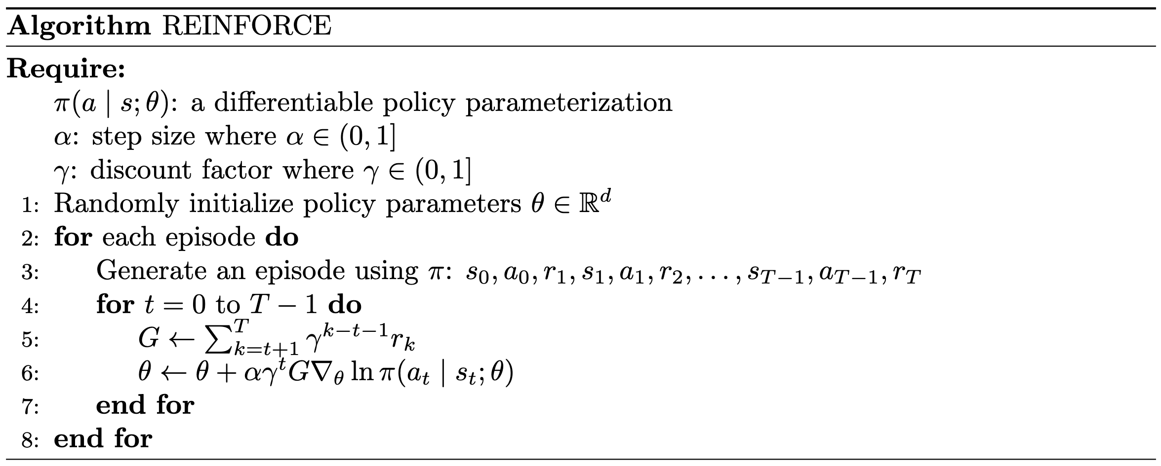
REINFORCE

Policy gradient algorithms seek a local maximum of \(J(\theta)\) by ascending its gradient with respect to \(\theta\) (Equation \(\eqref{eq:pg_grad}\)). However, the expression in Equation \(\eqref{eq:pgt}\) cannot be directly estimated using sampled trajectories, which is necessary for stochastic gradient methods. To address this, it can be re-expressed as follows:

\[ \begin{align*} \nabla_\theta J(\theta) &= \sum_{s \in \mathcal{S}} \mu(s) \sum_{a \in \mathcal{A}} Q_\pi(s, a) \nabla_\theta \pi(a \mid s; \theta) \\ &= \mathbb{E}_{s \sim \mu} \left[ \sum_{a \in \mathcal{A}} Q_\pi(s, a) \nabla_\theta \pi(a \mid s; \theta) \right] \;. \end{align*} \]

This formulation enables us to compute the policy gradient as an expectation, making it amenable to trajectory-based sampling. The update rule is then defined as:

\[ \begin{equation*} \theta_{t+1} = \theta_t + \alpha \sum_a Q_\pi(s_t, a) \nabla_\theta \pi(a \mid s_t; \theta) \;, \end{equation*} \]

This approach, however, requires summing over all possible actions, which can be computationally intractable or infeasible in many practical scenarios. Instead, we can reformulate the policy gradient by replacing the summation over all possible actions with an expectation under the policy \(\pi\), enabling us to sample from this expectation:

\[ \begin{align} \nabla_\theta J(\theta) &\propto \sum_{s \in \mathcal{S}} \mu(s) \sum_{a \in \mathcal{A}} Q_\pi(s, a) \nabla_\theta \pi(a \mid s; \theta) && \text{cf. Equation } \eqref{eq:pgt} \nonumber \\ &= \sum_{s \in \mathcal{S}} \mu(s) \sum_{a \in \mathcal{A}} Q_\pi(s, a) \frac{\pi(a \mid s; \theta)}{\pi(a \mid s; \theta)} \nabla_\theta \pi(a \mid s; \theta) \nonumber \\ &= \sum_{s \in \mathcal{S}} \mu(s) \sum_{a \in \mathcal{A}} Q_\pi(s, a) \pi(a \mid s; \theta) \frac{\nabla_\theta \pi(a \mid s; \theta)}{\pi(a \mid s; \theta)} \nonumber \\ &= \mathbb{E}_{s \sim \mu, a \sim \pi(\cdot \mid s; \theta)} \left[ Q_\pi(s_t, a_t) \frac{\nabla_\theta \pi(a_t \mid s_t; \theta)} {\pi(a_t \mid s_t; \theta)} \right] \nonumber \\ &= \mathbb{E}_{s \sim \mu, a \sim \pi(\cdot \mid s; \theta)} \left[ Q_\pi(s_t, a_t) \nabla_\theta \ln \pi(a_t \mid s_t; \theta) \right] \nonumber \\ &= \mathbb{E}_\pi \left[ G_t \nabla_\theta \ln \pi(a_t \mid s_t; \theta) \right] \label{sampled-gradient} \;, \end{align} \]

The Log-derivative Trick

The derivation of the sampled expectation for the policy gradient relies on a convenient identity, often referred to as the log-derivative trick. Fundamentally, this identity is an application of the chain rule for derivatives, which states:

\[ \begin{equation*} \frac{d}{dx}[f(g(x))] = f’(g(x)) g’(x). \end{equation*} \]

Applying this to the logarithmic function \(\ln(\pi(a_t \mid s_t; \theta))\), we have:

\[ \begin{align*} \nabla_\theta \big[ \ln \big( \pi(a_t \mid s_t; \theta) \big) \big] &= \frac{1}{\pi(a_t \mid s_t; \theta)} \nabla_\theta \pi(a_t \mid s_t; \theta) && \text{since } \frac{d}{dx}\ln(x) = \frac{1}{x} \\ &= \frac{\nabla_\theta \pi(a_t \mid s_t; \theta)}{\pi(a_t \mid s_t; \theta)} \;. \end{align*} \]

\[ \begin{equation*} \theta_{t+1} = \theta_t + \alpha G_t \nabla_\theta \ln \pi(a_t \mid s_t; \theta) \;. \end{equation*} \]

Note that, as expressed in Equation \(\eqref{sampled-gradient}\), the expectation of \(G_t \nabla_\theta \ln \pi(a_t \mid s_t; \theta)\) is proportional to, but not equal to, the true gradient of our objective \(\nabla_\theta J(\theta)\). Importantly, because the expectation of the sample gradient is proportional to the true gradient, the constant of proportionality can be absorbed into the step size \(\alpha\). Since \(\alpha\) is an arbitrary parameter, this flexibility simplifies the learning process without affecting convergence.

To establish the intuition for this update rule, we can revert the log-derivative trick and rearrange terms as follows:

\[ \begin{align} \theta_{t+1} &= \theta_t + \alpha G_t \nabla_\theta \ln \pi(a_t \mid s_t; \theta) \nonumber \\ &= \theta_t + \alpha G_t \frac{\nabla_\theta \pi(a_t \mid s_t; \theta)}{\pi(a_t \mid s_t; \theta)} \nonumber \\ &= \theta_t + \alpha \nabla_\theta \pi(a_t \mid s_t; \theta) \frac{G_t}{\pi(a_t \mid s_t; \theta)} \;. \label{eq:intuitive-update} \end{align} \]

From Equation \(\eqref{eq:intuitive-update}\), we observe that the update adjusts the policy parameters in the direction of \(\nabla_\theta \pi(a_t \mid s_t; \theta)\), which corresponds to increasing the probability of selecting action \(a_t\) in future visits to state \(s_t\). The magnitude of this adjustment is proportional to the return \(G_t\) and inversely proportional to the action probability \(\pi(a_t \mid s_t; \theta)\). Scaling by the return ensures that actions yielding higher returns have a greater influence on parameter updates. This causes the parameters to shift most significantly in directions that favor actions associated with higher rewards, effectively aligning the policy with desirable outcomes. The inverse proportionality to the action probability, on the other hand, corrects for the natural bias towards frequently selected actions. Without this normalization, actions with inherently higher probabilities (even if suboptimal) would dominate the updates due to being sampled more often. This adjustment ensures that the updates are weighted fairly, accounting for both the return and the likelihood of the action, thereby preventing suboptimal actions from disproportionately influencing the policy.

The Continuing Case

As noted earlier, the value function cannot serve as the objective function in the continuing case because it depends on a starting state. In an environment that proceeds infinitely, the influence of the starting state vanishes asymptotically. Consequently, we instead use the average reward per time step as the objective function:

\[ \begin{align} J(\theta) = R(\pi) &= \lim_{H \rightarrow \infty} \frac{1}{H} \sum_{t=1}^H \mathbb{E} \left[ r_t \mid s_0, a_{0:t-1} \sim \pi \right] \nonumber \\ &= \lim_{t \rightarrow \infty} \mathbb{E} \left[ r_t \mid s_0, a_{0:t-1} \sim \pi \right] \label{eq:ar2} \\ &= \sum_s \mu_\pi(s) \sum_a \pi(a \mid s) R(s,a) \;, \label{eq:ar3} \end{align} \]

where \(H\) is the horizon length, \(\mu_\pi(s)\) is the on-policy distribution, and the expectations are computed given the initial state \(s_0\) and the sequence of actions \(a_{0:t-1} = a_0, a_1, \dots, a_{t-1}\) generated by policy \(\pi\).

The equivalence of Equation \(\eqref{eq:ar2}\) and Equation \(\eqref{eq:ar3}\) holds when the MDP is ergodic, meaning a steady-state distribution:

\[ \begin{equation*} \sum_s \mu_\pi(s) \sum_a \pi(a \mid s) P(s’ \mid s,a) = \mu_\pi(s’) \;, \end{equation*} \]

exists and is independent of \(s_0\). In an ergodic MDP, the influence of the initial state and early actions diminishes over time. Thus, in the long run, the likelihood of being in any given state depends only on the policy \(\pi\) and the MDP's transition dynamics. This characteristic ensures that the average reward formulation accurately captures the expected behavior of the system as the horizon tends towards infinity.

The proof of the Policy Gradient Theorem for the continuing case is fundamentally the same as in the episodic case. For the full proof see chapter 13.6 in Reinforcement Learning: An Introduction (2018) by Richard S. Sutton and Andrew G. Barto.

Policy Gradients

The Policy Gradient Theorem

REINFORCE

The Continuing Case

References

- Reinforcement Learning: An Introduction (2018)
Richard S. Sutton and Andrew G. Barto
- Policy Gradient, Lectures on Reinforcement Learning (2015)
David Silver
- Policy Gradient Algorithms (2018)
Lilian Weng
- Policy Gradients (2021)
Sergey Levine
- Going Deeper Into Reinforcement Learning: Fundamentals of Policy Gradients (2017)
Daniel Seita
- Advanced Policy Gradient Methods (2017)
Joshua Achiam
- Log-derivative trick (2020)
Andy Jones
- The Reparameterization Trick (2018)
Gregory Gundersen
- Reparametrization Trick (2018)
Gabriel Huang