Prediction with Function Approximation

In model-free prediction, reinforcement learning algorithms update value estimates based on a backup value or update target. TD learning, for example, uses the target \(Y_t = r_{t+1} + \gamma V(s_{t+1})\). Practically, this means storing \(V(s)\) for each state \(s \in \mathcal{S}\) in a lookup table, hence the term “tabular methods.” This explicit representation of all state values becomes intractable for large or infinite state spaces. By estimating the value function, approximation methods offer a scalable alternative.

The Prediction Objective

In the tabular setting, state updates are independent and the value function provably converges to the true value function. These guarantees do not hold with function approximation. Nevertheless, our objective remains unchanged: to estimate expected returns for each state. To find optimal value function estimates, we must first formalize our optimization criterion. A canonical choice is the mean squared value error:

\[ \begin{equation}\label{eq:mean_square_error} \overline{\text{VE}}(\theta) = \sum_{s \in \mathcal{S}} \mu(s) \left[V(s) - \hat{V}(s; \theta) \right]^2 \;, \end{equation} \]

where \(\mu(s)\) is a state distribution with \(\mu(s) \geq 0\) and \(\sum_s \mu(s) = 1\), \(\theta\) is a parameter vector with \(|\theta| < |\mathcal{S}|\), and \(\hat{V}(s; \theta)\) approximates the true value function at state \(s\). The distribution \(\mu(s)\) weights each state's error contribution, reflecting the need to prioritize minimizing errors in certain states, as it is generally impossible to reduce error to zero across all states.

Ideally, we would like to find a global minimum \(\theta^*\) where \(\overline{\text{VE}}(\theta^*) \leq \overline{\text{VE}}(\theta)\) for all \(\theta\), but nonlinear function approximators generally lack global optimality guarantees. Even local minima — where the inequality holds in a neighborhood of \(\theta^*\) — are not guaranteed in RL, nor is bounded-distance convergence to any optimum. Despite lacking theoretical optimality guarantees, the MSE criterion \(\eqref{eq:mean_square_error}\) remains the practical choice for minimizing \(\overline{\text{VE}}\).

The on-policy distribution

The state distribution \(\mu(s)\) typically represents the fraction of time spent in each state. Under on-policy training, this is referred to as the on-policy distribution. For continuing tasks, this corresponds to the stationary distribution under policy \(\pi\) — the stable probability distribution over states that emerges as the agent follows \(\pi\) indefinitely. In other words, given sufficient time under a fixed policy, the probability of the agent being in each state stabilizes to a constant value.

For episodic tasks, the initial state distribution introduces bias in \(\mu(s)\) as the initial state \(s\) affects the proportion of time spent in each state. Let \(\rho(s)\) be the probability of starting an episode in state \(s\), \(\eta(s)\) be the expected time steps spent in \(s\) per episode, and \(\bar{s}\) be the predecessor state of \(s\). Then:

\[ \begin{align*} \eta(s) &= \mathbb{E}\left[ \sum_{t=0}^\infty \mathbf{1}_{s_t=s} \right] \\ &= \sum_{t=0}^{\infty} \mathbb{P}\left( s_t=s \right) \\ &= \mathbb{P}(s_0=s) + \sum_{t=1}^{\infty} \mathbb{P}(s_t=s) \\ &= \rho(s) + \sum_{t=1}^{\infty} \sum_{\bar{s}} P_\pi(s \mid \bar{s}) \mathbb{P}(s_{t-1}=\bar{s}) \\ &= \rho(s) + \sum_{\bar{s}} P_\pi(s \mid \bar{s}) \sum_{t=1}^{\infty} \mathbb{P}(s_{t-1}=\bar{s}) \\ &= \rho(s) + \sum_{\bar{s}} P_\pi(s \mid \bar{s}) \eta(\bar{s}) \\ &= \rho(s) + \sum_{\bar{s}} \eta(\bar{s}) \sum_{a} \pi(a \mid \bar{s}) P(s \mid \bar{s}, a) && \forall s \in \mathcal{S} \;. \end{align*} \]

The on-policy distribution \(\mu(s)\) is then obtained by normalizing \(\eta(s)\):

\[ \begin{align*} \mu(s) = \frac{\eta(s)}{\sum_{s’} \eta(s’)} && \forall s \in \mathcal{S} \;. \end{align*} \]

Stochastic Semi-Gradient Descent

Direct minimization of \(\overline{\text{VE}}(\theta)\) by enumerating \(\mathcal{S}\) is infeasible for large state spaces. Instead, we iteratively sample pairs \((s_t, V_\pi(s_t))\) where states \(s_t\) are drawn according to the same distribution \(\mu\) over which we are trying to minimize \(\overline{\text{VE}}\). While these samples may come from successive environmental states, this is not required.

We optimize \(\theta\) using stochastic gradient descent (SGD). Here, \(\theta \in \mathbb{R}^d\) is a column vector and \(\hat{V}(\theta)\) is a differentiable function with respect to \(\theta\) for all \(s \in \mathcal{S}\). SGD minimizes \(\overline{\text{VE}}(\theta)\) by iteratively adjusting \(\theta\) in the direction of steepest descent (i.e, the direction in which the error defined in Equation \(\eqref{eq:mean_square_error}\) is minimized most quickly):

\[ \begin{align} \theta_{t+1} &= \theta_t - \frac{1}{2} \alpha \nabla \left[ V_\pi(s_t) - \hat{V} (s_t; \theta_t) \right]^2 \label{eq:sgd1} \\ &= \theta_t + \alpha \Big[ V_\pi(s_t) - \hat{V}(s_t; \theta_t) \Big] \nabla \hat{V} (s_t; \theta_t) && \text{by the chain rule,} \label{eq:sgd2} \end{align} \]

where \(\theta_t\) is the weight vector at time step \(t\), \(\alpha\) is the step-size parameter, and \(\nabla \hat{V}(s_t;\theta_t)\) is the gradient of the approximate value function with respect to its parameters \(\theta_t\), evaluated at state \(s_t\). The gradient is the column vector of partial derivatives (see backpropagation note for details):

\[ \begin{equation*} \nabla \hat{V}(s; \theta) = \left[\frac{\partial \hat{V}(s; \theta)}{\partial \theta_1}, \frac{\partial \hat{V}(s; \theta)} {\partial \theta_2}, \dots, \frac{\partial \hat{V}(s; \theta)}{\partial \theta_n}\right]^\top \;. \end{equation*} \]

The purpose of \(\alpha\)

The step-size parameter \(\alpha\) governs the magnitude of updates to the parameter vector \(\theta\). While it might seem intuitive to fully minimize the error for each sampled state-value pair \((s_t, V_\pi(s_t))\), this approach would be suboptimal. Our objective is to minimize \(\overline{\text{VE}}\) across the entire state space, and generally, no parameter vector \(\theta\) exists that can achieve zero error for all states simultaneously — or even for all sampled states. Moreover, the approximate value function \(\hat{V}(\theta)\) must generalize beyond the sampled states, which are drawn stochastically (hence “stochastic” in SGD). By using a smaller step size, we allow \(\theta\) to find parameters that balance errors across the state space, promoting better generalization to unseen states. Fully correcting each sample would prevent this balance from emerging, as each update would override the compromises reached from previous samples.

In Equation \(\eqref{eq:sgd2}\), the update target \(Y_t\) is the true value function \(V\), which is typically unknown — hence the need for approximation. Importantly, convergence to a local optimum is guaranteed when using an unbiased estimator of \(V\) and a decreasing learning rate \(\alpha\) satisfying the Robbins-Monro conditions:

\[ \begin{align*} \sum_{n=1}^\infty \alpha_n &= \infty \;, && \sum_{n=1}^\infty \alpha^2_n < \infty \;. \end{align*} \]

The first condition ensures steps remain sufficiently large to overcome initial conditions and random fluctuations, allowing meaningful value estimate adjustments if, for example, the initial estimate is far from the true value. The second condition ensures convergence by gradually reducing step sizes until updates effectively cease; without this, persistent random fluctuations would prevent stabilization to an optimal value.

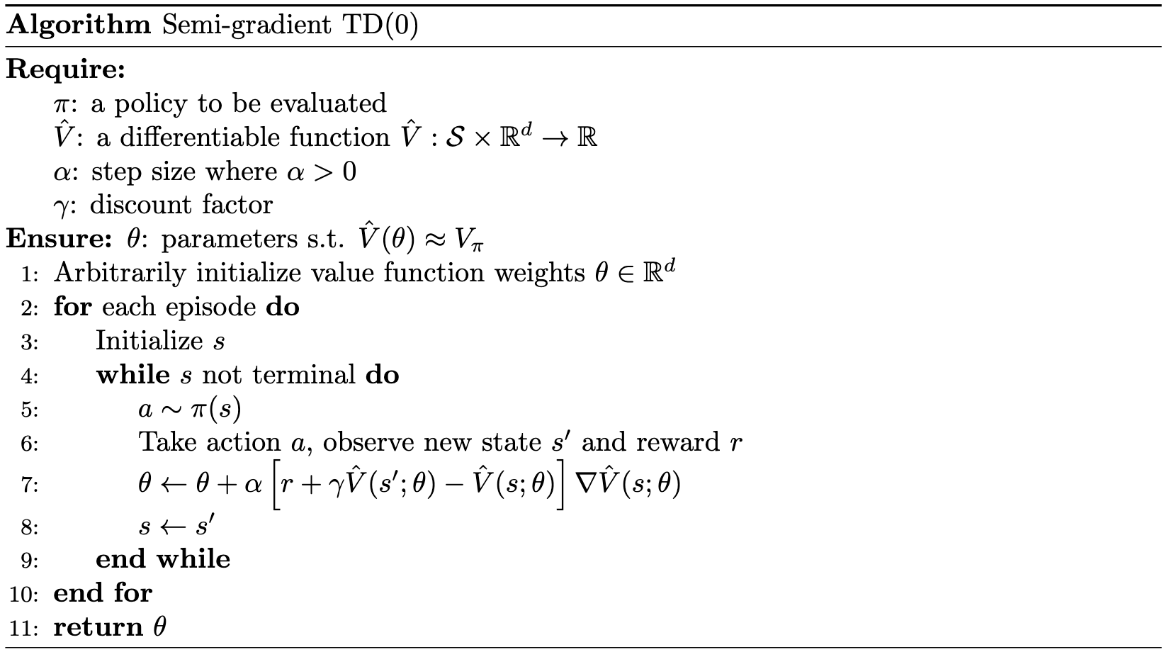
In Monte Carlo (MC) methods, the update target \(Y_t = G_t\) provides an unbiased estimate of \(V_\pi(s_t)\) as \(\mathbb{E}[G_t \mid s_t = s] = V_\pi(s) \; \forall t\). Temporal difference (TD) methods, by contrast, introduce bias due to bootstrapping. More specifically, this bias arises because the TD target \(Y_t = r_{t+1} + \gamma \hat{V}(s_{t+1}; \theta_t)\) is a function of \(\theta_t\) and is thus a “moving target”. When \(\theta\) is updated to minimize the error between \(Y_t\) and \(\hat{V}\), the change also affects our target value.

The use of boostrapping also has implications for the gradient computation. While a complete gradient calculation would require accounting for how updates to \(\theta\) affect both \(\hat{V}\) and \(Y_t\), the gradient through the target is omitted in Equation \(\eqref{eq:sgd2}\). To illustrate this missing gradient more clearly, we can substitute TD’s update target \(Y_t = r_{t+1} + \gamma \hat{V}(s_{t+1}; \theta_t)\) for \(V_\pi\) in Equation \(\eqref{eq:sgd1}\). Notice that the gradient of the squared error equals the TD update only when \(\nabla Y_t = 0\):

\[ \begin{align*} \frac{1}{2} \nabla \left[ Y_t - \hat{V}(s_t; \theta_t) \right]^2 &= \left(Y_t - \hat{V}(s_t; \theta_t) \right) \left( \nabla Y_t - \nabla \hat{V}(s_t; \theta_t) \right) && \text{by the chain rule} \\ &= -\left(Y_t - \hat{V} (s_t; \theta_t) \right) \nabla \hat{V}(s_t;\theta_t) && \text{iff } \nabla Y_t = 0; \text{cf. Equation } \eqref{eq:sgd2} \;. \end{align*} \]

\[ \begin{equation*} \nabla Y_t = \nabla \Big(r_{t+1} + \gamma \hat{V}(s_{t+1}; \theta_t) \Big) = \gamma \nabla \hat{V}(s_{t+1}; \theta_t) \neq 0 \;. \end{equation*} \]

This non-zero gradient means TD performs “semi-gradient” rather than true gradient descent on the squared error. While semi-gradient methods lack the convergence guarantees of true gradient descent, they often converge reliably in practice. True gradient descent could be achieved by applying the chain rule to allow a gradient through the target \(\nabla Y_t\), yielding residual gradient algorithms (see the off-policy control with function approximation note), but these typically perform poorly due to ill-conditioning.

Linear Methods

\[ \begin{equation}\label{eq:values_to_estimate} \hat{V}(s; \theta) = \sum_{i=0}^{d-1} \theta_i \phi_i(s) = \theta^\top \phi(s) \;, \end{equation} \]

where \(\phi : \mathcal{S} \rightarrow \mathbb{R}^d\) maps states to \(d\)-dimensional feature vectors. Each component \(\phi_i(s)\) of vector \(\phi(s)\) is a feature of state \(s\), and each function \(\phi_i : \mathcal{S} \rightarrow \mathbb{R}\) is a basis function (so named because the features form a linear basis for the set of approximate functions).

The gradient \(\nabla \hat{V}(s_t; \theta_t)\) reduces to the feature vector \(\phi(s_t)\), as the rate of change of \(\hat{V}(s_t; \theta_t)\) with respect to \(\theta\) depends only on the feature vector (see Equation \(\eqref{eq:values_to_estimate}\)). This mathematical simplification leads to a more concise form of the stochastic gradient descent update rule in equation \(\eqref{eq:sgd2}\):

\[ \begin{equation*} \theta_{t+1} = \theta_t + \alpha \left[ Y_t - \hat{V} (s_t; \theta_t) \right] \phi(s_t) \;. \end{equation*} \]

Basis Functions

The basis functions \(\phi_i\) should be simple to compute yet expressive enough to accurately approximate the value function through their linear combination. The choice of basis functions shapes what relationships can be captured. For example, consider a case in which states have two numerical dimensions, \(s_1 \in \mathbb{R}\) and \(s_2 \in \mathbb{R}\). The simplest representation \(\phi(s) = (s_1,s_2)^\top\) is restrictive in two ways. First, it cannot account for interactions between the components (e.g., the presence of \(s_1\) is good only in the absence of \(s_2\)) and second, if both \(s_1\) and \(s_2\) are zero, the estimated value would necessarily be zero. These limitations can be overcome with the addition of two features \(\phi(s) = (1,s_1,s_2,s_1s_2)^\top\). In fact, we can construct higher-dimensional feature vectors to account for even more complex relationships between the components \(\phi(s) = (1,s_1,s_2,s_1s_2,s_1^2,s_2^2,s_1^2s_2,s_1s_2^2,s_1^2s_2^2)^\top\). This method — referred to as the polynomial method — can be generalized beyond two components:

\[ \begin{equation} \nonumber \phi_i(s) = \prod_{j=1}^{k} s_j^{c_{i,j}} \;, \end{equation} \]

where \(k\) is the number of components \(s_1,s_2,\dots,s_k\) of each state \(s\), and \(c_{i,j}\) is an integer in the set \(\{0,1,\dots,n\}\) where \(n \geq 0\).

While higher-order polynomial bases allow for more complex relationships between features, the number of features grows exponentially with \(k\). This problem is not unique to the polynomial construction — many sophisticated methods such as tensor product constructions, state aggregation, and tile coding also suffer from the curse of dimensionality. In practice, the actual problem complexity is often lower than the complexity initially predicted by a human expert. This motivates the use of specialized automated feature selection methods developed for RL, which can significantly improve computational tractability.

Features for linear methods

To illustrate the concept of features, consider Tetris, a game with approximately \(10^{62}\) states that can be represented using 22 canonical basis functions:

Ten features mapping each state to individual column heights
Nine features mapping each state to adjacent column height differences
One feature mapping each state to the maximum column height
One feature counting board “holes”
One constant feature (equal to 1 for all states) enabling affine transformations

Beyond Linear Methods

In general, any function approximator can be used to estimate the value function \(\hat{V}(\theta)\). For instance, we can use a quadratic function \(\hat{V}(s; \theta) = \theta_0 + \theta_1\phi_1(s) + \theta_2\phi_1(s)^2\) or a higher-order polynomial \(\hat{V}(s; \theta) = \theta_0 + \theta_1\phi_1(s) + \theta_2\phi_1(s)^2 + \theta_3\phi_1(s)^3 + \dots\). However, as discussed in various notes including Deep Q-learning and Policy Gradients, most modern RL methods use a neural network function approximator.

References

- Reinforcement Learning: An Introduction (2018)
Richard S. Sutton and Andrew G. Barto
- Algorithms for Reinforcement Learning, Synthesis Lectures on Artificial Intelligence and Machine Learning (2019)
Csaba Szepesvari
- Reinforcement Learning: An Introduction (1998)
- Function Approximation, UC Berkeley CS287 Advanced Robotics (2019)
Pieter Abbeel
- Gradient Descent for General Reinforcement Learning, (1999)
Leemon Baird and Andrew Moore
- Artificial Intelligence: A Modern Approach, 4th edition (2020)
Stuart Russell and Peter Norvig
- An analysis of temporal-difference learning with function approximation (1997)
John N. Tsitsiklis and Benjamin Van Roy
- A Natural Policy Gradient (2001)
Sham Kakade
- Tetris: A Study of Randomized Constraint Sampling (2006)
Vivek F. Farias and Benjamin Van Roy
- Deriving the formula for the on policy distribution in episodic-tasks (2019)
David Rosenberg
- Deep RL with Q-Functions (2022)
Sergey Levine
- Model Free Control, Lectures on Reinforcement Learning (2015)