Constrained Markov Decision Processes
Revised August 13, 2025
The Markov Decision Processes note is optional but recommended background reading.
Reinforcement learning problems are typically formalized as the optimal control of an incompletely known Markov Decision Process (MDP), in which an agent seeks to maximize expected cumulative discounted reward:
\[ \begin{equation*} \text{arg} \max_{\pi \in \Pi} J^\pi = \mathbb{E}_{s \sim \mu, \tau \sim \pi} \left[ \sum_{t=0}^T \gamma^t r_t \right] = \sum_{s \in \mathcal{S}} \mu(s) V^\pi(s) \; . \end{equation*} \]
where \(\pi \in \Pi\) is a policy and \(\mu\) is an initial state distribution.
In many real-world settings, policies must not only maximize reward but also satisfy auxiliary constraints, such as limits on cost, risk, or safety violations. Constrained Markov Decision Processes (CMDPs) model such problems by introducing a set of cost functions \(\mathcal{C} = \{ C_1, \dots, C_m \}\) and corresponding bounds \(\mathbf{l} = \{ l_1, \dots, l_m \}\), where each \(C_i : \mathcal{S} \times \mathcal{A} \rightarrow \mathbb{R}\) and \(l_i \in \mathbb{R}\).
More formally, define the state-cost function as:
\[ \begin{equation*} V_{C_i}^\pi(s) = \mathbb{E}_{\tau \sim \pi} \left[ \sum_{t=0}^T \gamma^t C_i(s_t, a_t) \mid s_0 = s \right] \; , \end{equation*} \]
and the expected discounted cost under initial state distribution \(\mu\) as:
\[ \begin{equation*} J_{C_i}^\pi = \sum_{s \in \mathcal{S}} \mu(s) V_{C_i}^\pi(s) \; . \end{equation*} \]
The CMDP objective is:
\[ \begin{equation*} \arg\max_{\pi \in \Pi_C} J^\pi , \quad \text{where} \quad \Pi_C = \{ \pi \in \Pi : J_{C_i}^\pi \le l_i \ \forall i \} . \end{equation*} \]
Equivalently, writing the constraints explicitly gives:
\[ \begin{align}\label{eq:constrained} &\arg\max_{\pi \in \Pi} \; \sum_{s \in \mathcal{S}} \mu(s) V^\pi(s) \\ &\text{subject to} \quad \sum_{s \in \mathcal{S}} \mu(s) V_{C_i}^\pi(s) \leq l_i \quad \forall i \; . \nonumber \end{align} \]
Because strictly enforcing the constraints at every step of the optimization is typically computationally intractable, Equation \(\eqref{eq:constrained}\) is approximated with a regularized, unconstrained objective:
\[ \begin{equation}\label{eq:soft-penalties} \max_{\pi \in \Pi} \; J^\pi - \sum_{i=1}^m w_i \, [\, J_{C_i}^\pi - l_i \, ]_+ \;, \end{equation} \]
where \(w_i \ge 0\) are fixed penalty coefficients. The hinge form \([x]_+ = \max\{x,0\}\) ensures that penalties are applied only when a constraint is violated, preserving the intended semantics of the original problem. The naive form without \([\,\cdot\,]_+\) incorrectly rewards driving \(J_{C_i}^\pi\) far below \(l_i\).
While the soft penalties in Equation \(\eqref{eq:soft-penalties}\) avoid explicit constraint handling, they have significant drawbacks. First, they provide no guarantee that the final policy is feasible (i.e., respects all constraints). Second, performance is sensitive to the scaling and tuning of the penalty coefficients. Third, mixing reward and penalty terms in the objective can cause gradient interference, often leading to slow convergence or plateaus.
Lagrangian Relaxation
The limitations of fixed soft penalties motivate replacing hand-tuned weights with optimization-driven multipliers. Lagrangian relaxation introduces dual variables \(\lambda_i \ge 0\) that penalize violations adaptively rather than via preset \(w_i\), separating reward maximization from constraint enforcement and yielding a principled saddle-point problem. In what follows, the constrained objective is recast from a maximization (Equation \(\eqref{eq:soft-penalties}\)) to a minimization for alignment with standard optimization theory.
A generic constrained optimization problem:
\[ \begin{align}\label{eq:constrained-optimization} &\min_{\theta \in \mathbb{R}^d} L(\theta) \\ &\text{subject to} \quad C_i(\theta) - l_i \leq 0 \quad \forall i = 1, \dots, M \;, \nonumber \end{align} \]
can be relaxed by introducing penalty terms into the objective:
\[ \begin{equation*} \min_{\theta \in \mathbb{R}^d} \; \mathcal{L}(\theta, \lambda) = L(\theta) + \sum_{i=1}^M \lambda_i \left( C_i(\theta) - l_i \right) \; , \end{equation*} \]
where \(\lambda \in [0, \infty)^M\) is a vector of Lagrange multipliers.
The resulting function \(\mathcal{L}(\theta, \lambda)\) is the Lagrangian. This formulation “relaxes” the original problem by removing explicit constraints and instead penalizing constraint violations in the objective. If each \(\lambda_i\) is large enough, then any \(\theta\) that violates a constraint will yield a larger Lagrangian value than some feasible \(\theta\) with lower \(L(\theta)\), so the minimizer will prefer feasible solutions. This motivates the primal Lagrangian formulation:
\[ \begin{equation}\label{eq:primal} \mathcal{P}^* = \min_{\theta \in \mathbb{R}^d} \max_{\lambda \geq 0} \; \mathcal{L}(\theta, \lambda) = \min_{\theta \in \mathbb{R}^d} \max_{\lambda \geq 0} \left[ L(\theta) + \sum_{i=1}^M \lambda_i \left( C_i(\theta) - l_i \right) \right] \; . \end{equation} \]
Importantly, the constrained problem (Equation \(\eqref{eq:constrained-optimization}\)) and the primal Lagrangian (Equation \(\eqref{eq:primal}\)) share the same optimal solution \(\theta^*\) allowing \(\lambda_i \to \infty\). This equivalence can be seen by analyzing the inner maximization in Equation \(\eqref{eq:primal}\). If any constraint is violated (i.e., if \(C_i(\theta) - l_i > 0\) for some \(i\)) then the term \(\lambda_i \left( C_i(\theta) - l_i \right)\) grows without bound as \(\lambda_i \to \infty\), causing \(\mathcal{L}(\theta, \lambda)\) to diverge. Hence, the maximum over \(\lambda \geq 0\) is infinite whenever \(\theta\) is infeasible. To avoid this, any minimizing \(\theta\) must satisfy all constraints. Conversely, if \(\theta\) is feasible (i.e., \(C_i(\theta) - l_i \leq 0\) for all \(i\)), then the inner maximization is attained at \(\lambda = 0\), since each term \(\lambda_i \left( C_i(\theta) - l_i \right)\) is non-positive and thus maximized when \(\lambda_i = 0\). In that case, the Lagrangian reduces to \(L(\theta)\), and minimizing \(\mathcal{L}(\theta, \lambda)\) over feasible \(\theta\) is equivalent to minimizing \(L(\theta)\) subject to the constraints.
From the primal form, the Lagrangian dual is defined by reversing the order of optimization:
\[ \begin{equation*} \max_{\lambda \geq 0} \mathcal{D}(\lambda) = \max_{\lambda \geq 0} \min_{\theta \in \mathbb{R}^d} \mathcal{L}(\theta, \lambda) = \max_{\lambda \geq 0} \min_{\theta \in \mathbb{R}^d} \left[ L(\theta) + \sum_{i=1}^M \lambda_i \left( C_i(\theta) -l_i \right) \right] \; . \end{equation*} \]
Unlike the primal, the dual function \(\mathcal{D}(\lambda)\) is concave in \(\lambda\). This follows because \(\mathcal{L}(\theta, \lambda)\) is affine in \(\lambda\) for fixed \(\theta\), and \(\mathcal{D}(\lambda)\) is the pointwise minimum over a family of such affine functions. The pointwise minimum of concave functions is concave, and affine functions are both concave and convex; therefore, \(\mathcal{D}(\lambda)\) is concave.
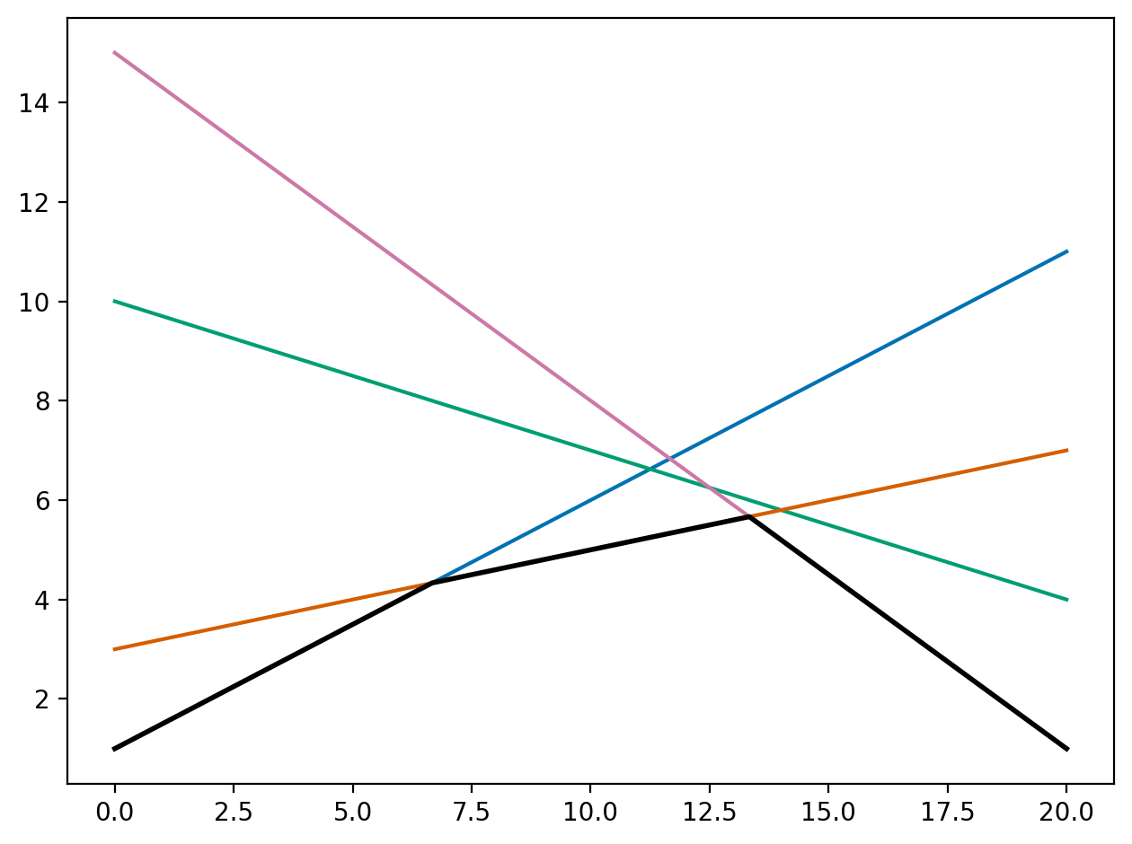 |
| Image adapted from StackExchange. The pointwise minimum of affine functions is concave. |
Because the dual objective \(\mathcal{D}(\lambda)\) is concave and the feasible set \(\{\lambda \in \mathbb{R}^M : \lambda \geq 0\}\) is convex, the dual problem is a convex optimization problem.
More specifically, by definition, a set \(S\) is convex if, for any \(u, v \in S\) and any \(\alpha \in [0,1]\), the point \(\alpha u + (1-\alpha)v\) is also in \(S\). To verify convexity of the feasible set, take \(\lambda^{(1)}, \lambda^{(2)}\) in the set. Then:
\[ \begin{equation*} \lambda^{(1)}, \lambda^{(2)} \in \mathbb{R}^M,\ \lambda^{(1)} \geq 0,\ \lambda^{(2)} \geq 0 \ \Rightarrow\ \alpha \lambda^{(1)} + (1 - \alpha) \lambda^{(2)} \color{red}{\geq} 0 \quad \forall \alpha \in [0, 1] \; . \end{equation*} \]
Since both \(\lambda^{(1)}\) and \(\lambda^{(2)}\) are componentwise nonnegative, each component of \(\alpha \lambda^{(1)} + (1 - \alpha) \lambda^{(2)}\) is a convex combination of nonnegative numbers and is therefore nonnegative, establishing the inequality \(\alpha \lambda^{(1)} + (1 - \alpha) \lambda^{(2)} \color{red}{\geq} 0\). Thus \(\alpha \lambda^{(1)} + (1 - \alpha) \lambda^{(2)}\) lies in the feasible set, and the set is convex.
The primal problem in Equation \(\eqref{eq:primal}\), by contrast, is generally not a convex optimization problem because the objective \(L(\theta)\) and constraint functions \(C_i(\theta)\) may be non-convex. Minimizing a non-convex function over the convex domain \(\mathbb{R}^d\) can yield multiple local minima, and standard convex optimization guarantees do not apply.
Although convex, the dual provides only a lower bound on the optimal value of the primal:
\[ \begin{equation*} \max_{\lambda \geq 0} \mathcal{D}(\lambda) = \max_{\lambda \geq 0} \min_{\theta \in \mathbb{R}^d} \mathcal{L}(\theta,\lambda) \leq \min_{\theta \in \mathbb{R}^d} \max_{\lambda \geq 0} \mathcal{L}(\theta,\lambda) = p^* \; . \end{equation*} \]
Here,
\[ \begin{equation*} p^* = \min_{\theta \in \mathbb{R}^d \,:\, C_i(\theta) \le l_i \ \forall i} L(\theta) \end{equation*} \]
denotes the optimal value of the original constrained problem in Equation \(\eqref{eq:constrained-optimization}\).
The Primal Formulation via Occupancy Measures
Solving the CMDP directly in the space of policies is difficult because the set of all possible policies is vast, and both the objective and constraints depend on the full distribution over trajectories they induce. However, the problem can be reformulated exactly by changing variables from a policy \(\pi\) to its induced discounted occupancy measure \(x\). This step relies on a structural property of CMDPs known as sufficiency: for any problem instance, there exists an optimal policy within the class of stationary policies. In the discounted occupancy measure space, the CMDP takes the form of a convex optimization problem, which admits a principled solution via Lagrangian duality.
Stationary Policies are Sufficient
The sufficiency of stationary policies can be shown by first defining the discounted normalized occupancy measure induced by a policy \(\pi\) and an initial distribution \(d_0\):
\[ \begin{equation}\label{eq:occupancy-measure} \phi_{d_0}^\pi(s,a) = (1 - \gamma) \sum_{t=0}^\infty \gamma^t \mathbb{P}[s_t = s, a_t = a \mid \pi, d_0] \;, \end{equation} \]
where the factor \((1 - \gamma)\) normalizes the distribution so that \(\sum_{s,a} \phi_{d_0}^\pi(s,a) = 1\).
The value function \(V_\pi(r, d_0)\) can be expressed in terms of the occupancy measure:
\[ \begin{align} (1 - \gamma) V_\pi(r, d_0) &= (1 - \gamma) \mathbb{E}_{d_0} \left[ \sum_{t=0}^\infty \gamma^t r(s_t, a_t) \right] && \text{by the definition of value function} \nonumber \\ &= (1 - \gamma) \sum_{t=0}^\infty \gamma^t \mathbb{E}_{d_0} [r(s_t, a_t)] && \text{by linearity of expectation} \nonumber \\ &= (1 - \gamma) \sum_{t=0}^\infty \gamma^t \sum_{s,a} \mathbb{P}[s_t = s, a_t = a \mid \pi, d_0] \, r(s,a) && \text{expanding the expectation} \nonumber \\ &= \sum_{s,a} \phi_{d_0}^\pi(s,a) \, r(s,a) && \text{by Equation } \eqref{eq:occupancy-measure} \nonumber \\ &= \langle \phi_{d_0}^\pi, r \rangle && \text{inner product notation} \label{eq:linear} \end{align} \]
Stationary policies are sufficient because, for any policy — including the optimal policy — there exists a stationary policy with an identical occupancy measure. Since the value function is linear in the occupancy measure (by Equation \(\eqref{eq:linear}\)), this implies equal expected return.
More formally, for any policy \(\pi\) and initial state distribution \(d_0\), there exists a stationary policy \(\pi'\) such that:
\[ \begin{equation}\label{eq:stationary-policy} \phi_{d_0}^\pi(s,a) = \phi_{d_0}^{\pi’}(s,a) \quad \forall (s,a) \;, \end{equation} \]
where \(\pi'\) is:
\[ \begin{equation}\label{eq:policy} \pi’(a \mid s) = \frac{\phi_{d_0}^\pi(s,a)}{\phi_{d_0}^\pi(s)} \;, \end{equation} \]
and \(\phi_{d_0}^\pi(s) = \sum_a \phi_{d_0}^\pi(s,a)\). If \(\phi_{d_0}^\pi(s) = 0\), any valid distribution over actions may be selected.
Intuitively, the definition in Equation \(\eqref{eq:policy}\) constructs a stationary policy by matching the conditional action probabilities observed under the original policy. The occupancy measure \(\phi_{d_0}^\pi(s,a)\) gives the long-run discounted frequency of visiting state–action pair \((s,a)\), while \(\phi_{d_0}^\pi(s)\) is the corresponding frequency of visiting state \(s\). Their ratio is therefore the empirical probability of taking action \(a\) when in state \(s\) under \(\pi\). Choosing \(\pi'\) to equal this ratio ensures that \(\pi'\) induces exactly the same occupancy measure as \(\pi\), and hence achieves identical objective value and constraint satisfaction.
Proving Stationary Policies are Sufficient
We now show that, given Equation \(\eqref{eq:policy}\), \(\phi_{d_0}^\pi(s) = \phi_{d_0}^{\pi’}(s)\) for all states \(s\), which immediately implies Equation \(\eqref{eq:stationary-policy}\). Let:
\[ \begin{equation}\label{eq:transition-probability} P^{\pi’}(s, s’) = \sum_{a} \pi’(a \mid s) \mathbf{P}(s, a, s’) \;, \end{equation} \]
denote the probability of transitioning to \(s'\) from \(s\) under policy \(\pi'\). Then:
\[ \begin{align*} \phi_{d_0}^\pi(s) &= (1 - \gamma) \sum_{t=0}^\infty \gamma^t \mathbb{P}[s_t = s \mid \pi, d_0] && \text{by Equation } \eqref{eq:occupancy-measure} \\ &= (1 - \gamma)d_0(s) + (1 - \gamma) \sum_{t=1}^\infty \gamma^t \mathbb{P}[s_t = s \mid \pi, d_0] && \text{isolate \(t=0\) term} \\ &= (1 - \gamma)d_0(s) + (1 - \gamma)\gamma \sum_{t=0}^\infty \gamma^t \mathbb{P}[s_{t+1} = s \mid \pi, d_0] && \text{reindex the sum} \\ &= (1 - \gamma)d_0(s) + \gamma \sum_{s’, a} \left[ (1 - \gamma) \sum_{t=0}^\infty \gamma^t \mathbb{P}[s_t = s’, a_t = a \mid \pi, d_0] \right] \mathbf{P}(s’, a, s) && \text{one-step expansion using total probability} \\ &= (1 - \gamma)d_0(s) + \gamma \sum_{s’, a} \phi_{d_0}^\pi(s’, a) \, \mathbf{P}(s’, a, s) && \text{by Equation } \eqref{eq:occupancy-measure} \\ &= (1 - \gamma)d_0(s) + \gamma \sum_{s’} \sum_a \phi_{d_0}^\pi(s’, a) \, \mathbf{P}(s’, a, s) && \text{reorder summation} \\ &= (1 - \gamma)d_0(s) + \gamma \sum_{s’} \left( \sum_a \frac{\phi_{d_0}^\pi(s’, a)}{\phi_{d_0}^\pi(s’)} \, \mathbf{P}(s’, a, s) \right) \phi_{d_0}^\pi(s’) && \text{multiply and divide by } \phi_{d_0}^\pi(s’) \\ &= (1 - \gamma)d_0(s) + \gamma \sum_{s’} \left( \sum_a \pi’(a \mid s’) \, \mathbf{P}(s’, a, s) \right) \phi_{d_0}^\pi(s’) && \text{by Equation} \eqref{eq:policy} \\ &= (1 - \gamma)d_0(s) + \gamma \sum_{s’} \phi_{d_0}^\pi(s’) \, P^{\pi’}(s’, s) && \text{by Equation } \eqref{eq:transition-probability} \end{align*} \]
Because the policy \(\pi'\) is fixed, the final expression can be written in vector form using a transition matrix \(P^{\pi’}\) and a row vector \(\phi_{d_0}^\pi\):
\[ \begin{equation*} \phi_{d_0}^\pi = (1 - \gamma)d_0 + \gamma \phi_{d_0}^\pi P^{\pi’} \;. \end{equation*} \]
Solving this recurrence:
\[ \begin{align*} \phi_{d_0}^\pi &= (1 - \gamma)d_0 + \gamma \phi_{d_0}^\pi P^{\pi’} \\ \phi_{d_0}^\pi - \gamma \phi_{d_0}^\pi P^{\pi’} &= (1 - \gamma)d_0 \\ \phi_{d_0}^\pi (\mathbf{I} - \gamma P^{\pi’}) &= (1 - \gamma)d_0 \\ \phi_{d_0}^\pi &= (1 - \gamma)d_0 (\mathbf{I} - \gamma P^{\pi’})^{-1} \;. \end{align*} \]
But this is exactly the solution to the linear system defined by the dynamics under \(\pi'\):
\[ \begin{align*} \phi_{d_0}^{\pi’} &= (1 - \gamma)d_0 + \gamma \phi_{d_0}^{\pi’} P^{\pi’} \\ \phi_{d_0}^{\pi’} (\mathbf{I} - \gamma P^{\pi’}) &= (1 - \gamma)d_0 \\ \phi_{d_0}^{\pi’} &= (1 - \gamma)d_0 (\mathbf{I} - \gamma P^{\pi’})^{-1} \;. \end{align*} \]
The matrix \(\mathbf{I} - \gamma P^{\pi’}\) is invertible because \(P^{\pi’}\) is stochastic (all row sums are \(1\)) and \(0 \le \gamma < 1\) ensures that \(\rho(\gamma P^{\pi’}) < 1\), where \(\rho(\cdot)\) denotes the spectral radius. Since \(\mathbf{I} - \gamma P^{\pi’}\) is invertible, the linear system:
\[ \begin{equation*} \phi(\mathbf{I} - \gamma P^{\pi’}) = (1 - \gamma)d_0 \end{equation*} \]
has exactly one solution for \(\phi\). Both \(\phi_{d_0}^\pi\) and \(\phi_{d_0}^{\pi’}\) satisfy this system. By uniqueness they must, therefore, be equal:
\[ \begin{equation*} \phi_{d_0}^\pi = \phi_{d_0}^{\pi’} \;. \end{equation*} \]
Thus, any occupancy measure induced by an arbitrary policy can be matched by that of a stationary policy. This establishes the sufficiency of stationary policies. The algebraic structure mirrors the matrix formulation of value functions in Markov reward processes, highlighting the close connection between occupancy measures and value functions.
The Equivalent Linear Program
From the sufficiency of stationary policies, any feasible policy in the CMDP defined in Equation \(\eqref{eq:constrained}\) can be replaced by a stationary policy with the same discounted occupancy measure. For a stationary policy \(\pi'\), the discounted occupancy measure \(x(s,a) = \phi_{d_0}^{\pi’}(s,a)\) satisfies the balance equation obtained by marginalizing Equation \(\eqref{eq:occupancy-measure}\) over \(a\) and expanding one step forward in time under the transition dynamics \(\mathbf{P}\):
\[ \begin{equation*} \sum_a x(s,a) = (1-\gamma)d_0(s) + \gamma \sum_{s’,a} x(s’,a)\,\mathbf{P}(s’,a,s) \quad \forall s \in \mathcal{S}. \end{equation*} \]
The set of all discounted occupancy measures achievable by some stationary policy is therefore
\[ \begin{equation*} X_\gamma = \left\{ x \in [0,\infty)^{\mathcal{S} \times \mathcal{A}} \; \middle| \; \sum_a x(s,a) = (1-\gamma)d_0(s) + \gamma \sum_{s’,a} x(s’,a) \mathbf{P}(s’,a,s),\; \forall s \in \mathcal{S} \right\} \;. \end{equation*} \]
Expressing the CMDP objective in terms of \(x\) yields an equivalent linear program:
\[ \begin{align} \min_{x} &\; -\langle x, r \rangle \label{eq:linear-program} \\ \text{s.t.} \quad &x \in X_\gamma \nonumber \\ &\langle x, C_i \rangle - (1-\gamma)l_i \leq 0, \quad i = 1, \dots, m \; . \nonumber \end{align} \]
The reward and cost constraints are linear in \(x\) because \(J^\pi\) and \(J_{C_i}^\pi\) are inner products between the occupancy measure and the corresponding reward or cost function (Equation \(\eqref{eq:linear}\)). The feasible set \(X_\gamma\) is defined by linear flow-conservation constraints, so the entire problem is a finite-dimensional linear program over the occupancy measure space.
The Lagrangian in Reinforcement Learning
In the CMDP linear program (Equation \(\eqref{eq:linear-program}\)), the Lagrangian is:
\[ \begin{align} \mathcal{L}(x,\lambda) &= -\langle x, r \rangle + \sum_{i=1}^m \lambda_i \left( \langle x, C_i \rangle - (1-\gamma) l_i \right) \label{eq:rl-lagrangian} \\ &= -\sum_{s,a} x(s,a) \, r(s,a) + \sum_{i=1}^m \lambda_i \left[ \sum_{s,a} x(s,a) \, C_i(s,a) - (1-\gamma) l_i \right] && \text{expand inner products: }\langle f, g \rangle = \sum_{s,a} f(s,a) g(s,a) \nonumber \\ &= -\sum_{s,a} x(s,a) \, r(s,a) + \sum_{i=1}^m \lambda_i \sum_{s,a} x(s,a) \, C_i(s,a) - (1-\gamma) \sum_{i=1}^m \lambda_i l_i && \text{distribute the sum over \(i\)} \nonumber \\ &= \sum_{s,a} x(s,a) \left[ -r(s,a) + \sum_{i=1}^m \lambda_i C_i(s,a) \right] - (1-\gamma) \sum_{i=1}^m \lambda_i l_i && \text{group reward and cost terms inside a single bracket} \nonumber \\ &= \left\langle x, -r + \sum_{i=1}^m \lambda_i C_i \right\rangle - (1-\gamma) \sum_{i=1}^m \lambda_i l_i && \text{rewrite in inner product notation} \nonumber \\ &= \langle x, r_\lambda \rangle - (1-\gamma) \sum_{i=1}^m \lambda_i l_i && \text{define } r_\lambda(s,a) = -r(s,a) + \sum_{i=1}^m \lambda_i C_i(s,a) \nonumber \end{align} \]
In the primal formulation:
\[ \begin{equation}\label{eq:rl-primal} \mathcal{P}^* = \min_{x \in X_\gamma} \; \max_{\lambda \geq 0} \; \mathcal{L}(x,\lambda) \;, \end{equation} \]
the maximization over \(\lambda\) enforces the CMDP constraints: if some \(k\) satisfies \(\langle x, C_k \rangle - (1-\gamma) l_k > 0\), then as \(\lambda_k \to \infty\) the Lagrangian diverges to \(+\infty\), so any minimizer of the outer problem must satisfy all constraints. Thus, if \(\lambda^*\) corresponding to an optimal occupancy \(x^*\) were given, one might attempt to recover \(x^*\) by solving:
\[ \begin{equation}\label{eq:minimization-problem} \min_{x \in X_\gamma} \mathcal{L}(x,\lambda^*) \;, \end{equation} \]
where
\[ \begin{align*} \mathcal{L}(x,\lambda^*) = \langle x, r_{\lambda^*} \rangle \color{red}{- (1-\gamma)\sum_{i=1}^m \lambda_i^* l_i} \quad \text{and} \quad r_{\lambda^*}(s,a) = -r(s,a) + \sum_{i=1}^m \lambda_i^* C_i(s,a) \;, \end{align*} \]
because the constant term (in red) does not affect the minimizer, Equation \(\eqref{eq:minimization-problem}\) is equivalent to the single-objective MDP:
\[ \begin{equation*} \max_{x \in X_\gamma} \langle x, -r_{\lambda^*} \rangle \;, \end{equation*} \]
which can be solved with standard RL methods.
However, solving a scalarized subproblem at fixed \(\lambda^*\) does not, in general, solve the original CMDP. Two structural issues prevent this reduction. First, minimizers at fixed \(\lambda^*\) are generally nonunique. The set \(\arg\min_{x \in X_\gamma} \mathcal{L}(x,\lambda^*)\) may contain occupancies corresponding to deterministic policies that cease to be optimal once \(\lambda\) is reoptimized. Second the constrained optimum can require stochastic stationary policies even when each scalarized subproblem admits a deterministic solution. A deterministic minimizer of \(\mathcal{L}(\cdot,\lambda^*)\) can therefore fail to satisfy the original CMDP constraints.
Uniformly Optimal Stationary Policies May Not Exist and Optimal Policies May Be Stochastic
While there exists a uniformly optimal, stationary policy in MDPs, in general this property does not hold in CMDPs.
Consider a two-state CMDP in which the agent, from state \(s_1\), transitions to \(s_1\) with probability \(p\) and to \(s_2\) with probability \(1 - p\). These transitions yield rewards of \(0\) and \(1\), and costs of \(0\) and \(1\), respectively. From \(s_2\), the agent deterministically remains in \(s_2\), collecting a reward of \(1\) and incurring a cost of \(-1\). In such a CMDP, any stationary policy is fully characterized by \(p \in [0, 1]\).
Without loss of generality, set \(\gamma = 0\). Let \(d_0 \in [0,1]\) denote the probability of starting in \(s_1\), defining the initial state distribution. For a stationary policy parameterized by \(p\), the expected reward and cost are:
\[ \begin{align*} V_p(r, d_0) &= d_0 \left( p \cdot 0 + (1 - p) \cdot 1 \right) + (1 - d_0)(1) \\ &= d_0(1 - p) + 1 - d_0 \;, \\ V_p(c, d_0) &= d_0 \left( p \cdot 0 + (1 - p) \cdot 1 \right) + (1 - d_0)(-1) \\ &= d_0(1 - p) - 1 + d_0 \;. \end{align*} \]
Let the constraint limit be \(\mathbf{l} = [0]\). Feasibility requires that the expected cost not exceed this limit:
\[ \begin{align*} V_p(c, d_0) &= d_0(1 - p) - 1 + d_0 \leq 0 \\ 2d_0 - d_0p - 1 &\leq 0 \\ -d_0p &\leq -2d_0 + 1 \\ p &\geq \frac{2d_0 - 1}{d_0} \end{align*} \]
This inequality characterizes the set of feasible stationary policies for each \(d_0\). When \(d_0 > 0.5\), the set of feasible stationary policies is \(p \in \left[\frac{2d_0 - 1}{d_0}, 1\right]\). Since \(V_p(r, d_0)\) is decreasing in \(p\), the reward-maximizing policy within this range is:
\[ \begin{equation*} p^* = \frac{2d_0 - 1}{\color{red}{d_0}} \;. \end{equation*} \]
Because this optimal value of \(p\) depends on \(d_0\), different initial state distributions induce different optimal policies. No single stationary policy is optimal for all \(d_0\), so no uniformly optimal stationary policy exists.
When \(d_0 > \frac{1}{2}\), the optimal stationary policy satisfies \(0 < p^* < 1\) and therefore randomizes between actions. Evaluating the reward at \(p^*\) using \(V_p(r, d_0) = d_0(1 - p) + 1 - d_0\) gives:
\[ \begin{equation*} V_{p^*}(r, d_0) = 2 - 2d_0 \;. \end{equation*} \]
The best deterministic stationary policy in this regime is \(p = 1\), which yields:
\[ \begin{equation*} V_{p=1}(r, d_0) = 1 - d_0 \;. \end{equation*} \]
The value difference:
\[ \begin{equation*} V_{p^*}(r, d_0) - V_{p=1}(r, d_0) = 1 - d_0 \end{equation*} \]
shows that restricting policies to be deterministic in this CMDP strictly reduces the achievable value by \(1 - d_0\) for every \(\frac{1}{2} < d_0 < 1\).
The correct solution must instead satisfy the saddle-point condition:
\[ \begin{equation*} \mathcal{L}(x^*,\lambda) \le \mathcal{L}(x^*,\lambda^*) \le \mathcal{L}(x,\lambda^*) \quad \forall x \in X_\gamma,\; \forall \lambda \ge 0, \end{equation*} \]
not merely optimality at a fixed \(\lambda^*\).
Rock–Paper–Scissors offers a simple analogy. The mixed strategy with uniform probabilities \(\lambda_1^* = \lambda_2^* = \lambda_3^* = 1/3\) is a Nash equilibrium. If the opponent is fixed to uniform play, any deviation leaves the payoff unchanged at \(0\). Once the opponent is allowed to reoptimize, however, that deviation becomes exploitable. Similarly, in CMDPs, minimizing \(\mathcal{L}(\cdot,\lambda^*)\) at fixed \(\lambda^*\) can appear neutral but is not valid unless \((x^*,\lambda^*)\) forms a saddle point stable to dual reoptimization.
Solving CMDPs
While a CMDP cannot, in general, be reduced to an equivalent unconstrained MDP by fixing \(\lambda^*\), the saddle-point formulation in Equation \(\eqref{eq:rl-primal}\) allows each primal update to be carried out by solving an unconstrained MDP. The optimal dual variables are given by \(\lambda_*(x) = \arg\max_{\lambda \ge 0} \mathcal{L}(x,\lambda)\). Danskin’s theorem implies that the gradient of the min–max objective with respect to \(x\) is equal to the partial derivative of \(\mathcal{L}\) with respect to \(x\), evaluated at any maximizer \(\lambda_*\). Thus, at a given \(x\), the primal update is identical to that of an unconstrained MDP with the reward function replaced by its \(\lambda_*(x)\)-weighted counterpart. Importantly, this is not a single fixed MDP but a sequence of unconstrained MDPs — one for each \(\lambda_*(x_k)\) encountered during the iterations—solved alongside the dual updates.
Danskin's Theorem
Let \(\mathcal{L}^\prime_x(x,\lambda)\) denote the partial derivative of \(\mathcal{L}(x,\lambda)\) with respect to \(x\). For fixed \(x\), let \(\lambda_*(x)\) be any maximizer of \(\mathcal{L}(x,\cdot)\), and define:
\[ \begin{equation*} \Phi(x) = \mathcal{L}(x, \lambda_*(x)). \end{equation*} \]
If \(\mathcal{L}\) is continuously differentiable in \(x\) for all \(\lambda\) and the maximizer \(\lambda_*(x)\) is unique, then:
\[ \begin{equation*} \nabla \Phi(x) = \mathcal{L}^\prime_x\big(x, \lambda_*(x)\big). \end{equation*} \]
Thus, the gradient of \(\Phi\) with respect to \(x\) can be evaluated by differentiating \(\mathcal{L}\) with respect to \(x\) at the dual optimizer \(\lambda_*(x)\), without differentiating through \(\lambda_*(x)\) itself. This property is useful in policy-gradient methods for CMDPs because it allows the primal update to be computed without explicitly tracking how the optimal multipliers change with the policy.
Using Gradient-Based Methods to Solve CMDPs
Danskin's theorem implies that the gradient of \(\Phi(x) = \mathcal{L}(x, \lambda_*(x))\) can be computed as \(\mathcal{L}_x^\prime(x,\lambda_*(x))\), where \(\lambda_*(x)\) maximizes \(\mathcal{L}(x, \cdot)\) for fixed \(x\). This allows the search for a saddle point to be formulated as the ordinary differential equation:
\[ \begin{equation}\label{eq:ode} \dot{x} = -\mathcal{L}_x^\prime(x,\lambda_*(x)). \end{equation} \]
However, \(\lambda_*(x)\) is not known explicitly. Thus, for fixed \(x\), a maximizer is computed by projected gradient ascent:
\[ \begin{equation}\label{eq:lambda-projected} \lambda^{k+1} = \Pi_{[0,\infty)^m}\!\left( \lambda^{k} + \eta_k \,\mathcal{L}_{\lambda}^\prime(x,\lambda^{k}) \right), \end{equation} \]
where \(\Pi_{[0,\infty)^m}\) denotes Euclidean projection onto the nonnegativity constraints and \(\eta_k > 0\) is a stepsize. The projection enforces \(\lambda^{k+1} \ge 0\) componentwise and the iterates converge to a maximizer \(\lambda_*(x)\) for any initial \(\lambda^0 \ge 0\).
To compute \(\Phi\), the dynamics (Equation \(\eqref{eq:ode}\)) and the projected gradient-ascent dynamics for \(\lambda\) (Equation \(\eqref{eq:lambda-projected}\)) can be combined into the coupled system
\[ \begin{align*} \dot{x} &= -\epsilon \, \mathcal{L}_x^\prime(x,\lambda) \\ \dot{\lambda} &= \Pi_{[0,\infty)^m}\!\left( \mathcal{L}_{\lambda}^\prime(x,\lambda) \right) \;, \end{align*} \]
where \(\epsilon\) is small so that updates to \(\lambda\) occur on a faster timescale than updates to \(x\).
This separation of timescales is necessary because \(\dot{x}\) depends on \(\lambda\), and accurate optimization of \(x\) requires that \(\lambda\) be close to \(\lambda_*(x)\). The \(\lambda\)-update is the inner-loop optimization, while the \(x\)-update is the outer-loop optimization. In practice, \(\lambda_*(x)\) may be unbounded and perfect separation is impossible, so a discrete two-timescale recursion is used instead:
\[ \begin{align*} x_{k+1} &= x_k - a_k \big( \mathcal{L}_x^\prime(x_k,\lambda_k) + W_k \big), \\ \lambda_{k+1} &= \Pi_{[0,\infty)^m} \!\left( \lambda_k + b_k \big( \mathcal{L}_{\lambda}^\prime(x_k,\lambda_k) + U_k \big) \right), \end{align*} \]
where \((a_k)\) and \((b_k)\) are positive step-size sequences with \(a_k \ll b_k\) and both \(a_k \to 0\), \(b_k \to 0\) at rates slow enough to ensure convergence. The terms \(W_k\) and \(U_k\) are zero-mean noise sequences.
Finally, since \(x\) is a discounted occupancy measure, directly updating \(x\) requires maintaining a distribution over all states, which is often impractical. Instead, the search can be carried out in a smoothly parameterized policy class \(\pi_\theta\). In this parameterized setting, the Lagrangian in Equation \(\eqref{eq:rl-lagrangian}\) becomes:
\[ \begin{align} \mathcal{L}(\theta,\lambda) &= -(1-\gamma) \, V_{\pi_\theta}(r,d_0) + \sum_{i=1}^m \lambda_i \left[ (1-\gamma) \, V_{\pi_\theta}( C_i, d_0 ) - (1-\gamma)l_i \right] \label{eq:rl-lagrange} \\ &= - (1-\gamma) \, V_{\pi_\theta} \left( r - \sum_{i=1}^m \lambda_i C_i, d_0 \right) - (1-\gamma) \sum_{i=1}^m \lambda_i l_i \;, \nonumber \end{align} \]
where \(V_{\pi_\theta}(f,d_0)\) denotes the \(\gamma\)-discounted value of signal \(f\) under \(\pi_\theta\) from initial distribution \(d_0\).
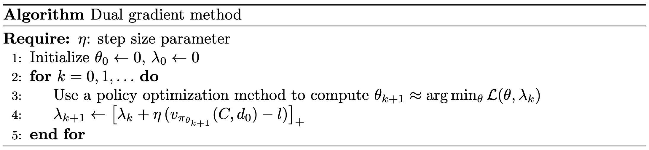
Gradient-Based Primal–Dual Methods for CMDPs
A constrained MDP requires simultaneous optimization over the primal parameters \(\theta\) and the nonnegative dual multipliers \(\lambda\). The optimization alternates between decreasing the Lagrangian with respect to \(\theta\) and increasing it with respect to \(\lambda\).
For the dual variables, the partial derivative of \(\mathcal{L}(\theta,\lambda)\) with respect to \(\lambda_i\) is
\[ \begin{equation}\label{eq:multipliers-update} \frac{\partial}{\partial \lambda_i} \mathcal{L}(\theta,\lambda) = (1-\gamma) \, V_{\pi_\theta}(C_i, d_0) - (1-\gamma) \, l_i, \end{equation} \]
which is positive when the \(i\)th cost exceeds its limit and negative otherwise. This update increases multipliers when constraints are violated and decreases them when they are satisfied.
For the primal parameters, fixing \(\lambda\) yields an unconstrained MDP with modified reward:
\[ \begin{equation*} r(s,a) - \sum_{i=1}^m \lambda_i C_i(s,a) \;, \end{equation*} \]
which can be optimized using any policy optimization method. In gradient-based primal–dual algorithms, \(\theta\) is updated to approximately minimize \(\mathcal{L}(\theta,\lambda)\) for the current \(\lambda\), and \(\lambda\) is updated by projected gradient ascent to preserve nonnegativity. This produces a sequence of unconstrained MDPs, each corresponding to the current multiplier vector, and converges to a saddle point under suitable step-size conditions.
 |
Because the dual objective lower bounds the primal objective, a zero duality gap guarantees that solving the dual yields the same optimal value as solving the primal directly. In the tabular setting, constrained reinforcement learning satisfies this property exactly. With parameterized policies, the duality gap is bounded linearly by the approximation error and can be reduced arbitrarily by increasing the representational capacity of \(\pi_\theta\).
Citation
Landers, Matthew. "Constrained Markov Decision Processes." mattlanders.net, August 13, 2025. mattlanders.net/constrained-mdps.
@article{landers2025constrainedmdps,
  title = {Constrained Markov Decision Processes},
  author = {Landers, Matthew},
  journal = {mattlanders.net},
  year = {2025},
  month = {August},
  url = "mattlanders.net/constrained-mdps"
}
References
- Constrained MDPs and the reward hypothesis (2020)
Csaba Szepesvari
- Cornell CS 5787: Applied Machine Learning. Lecture 10. Part 1: Lagrange Duality [video] (2021)
Volodymyr Kuleshov
- Constrained Reinforcement Learning Has Zero Duality Gap, Advances in Neural Information Processing Systems (2019)
Santiago Paternain, Luiz F. O. Chamon, Miguel Calvo-Fullana, and Alejandro Ribeiro
- Duality (2023)
Stephen Boyd
- An introduction to ordinary differential equations (2020)
Duane Q. Nykamp
- Convex Optimization (2015)
Ryan Tibshirani