Conjugate Gradient Method
Revised May 26, 2025
Consider a linear system of the form:
\[ \begin{equation}\label{eq:system-of-linear-equations} \mathbf{Ax} = \mathbf{b} \;, \end{equation} \]
where \(\mathbf{x}\) is an unknown vector, \(\mathbf{b}\) is a known vector, and \(\mathbf{A}\) is a known, square, symmetric, positive-definite matrix (i.e., for any non-zero vector \(\mathbf{z}\), \(\mathbf{z}^\top \mathbf{Az} > 0\)). Although such a system admits a closed-form solution:
\[ \begin{equation}\label{eq:closed-from-solution} \mathbf{x}^* = \mathbf{A}^{-1} \mathbf{b} \;, \end{equation} \]
directly computing \(\mathbf{A}^{-1}\) is computationally expensive and often numerically unstable, especially in large, sparse settings. In practice, iterative methods are preferred, as they avoid matrix inversion altogether. Such approaches are motivated by the observation that the solution \(\mathbf{x}^*\) can equivalently be characterized as the unique vector satisfying:
\[ \begin{equation}\label{eq:solution-condition} \mathbf{Ax}^* - \mathbf{b} = \mathbf{0} \;. \end{equation} \]
This suggests the solution can be found by minimizing a differentiable function \(f : \mathbb{R}^n \to \mathbb{R}\) such that \(\nabla f(\mathbf{x}) = \mathbf{Ax} - \mathbf{b}\). More specifically, any minimizer \(\mathbf{x}^*\) must satisfy the first-order optimality condition \(\nabla f(\mathbf{x}^*) = \mathbf{0}\). Substituting the expression \(\nabla f(\mathbf{x}^*) = \mathbf{Ax}^* - \mathbf{b}\) into this condition yields Equation \(\eqref{eq:solution-condition}\). Note that while a zero gradient is a necessary condition for any local extremum or saddle point, the strict convexity of \(f(\mathbf{x})\) — guaranteed by the symmetry and positive definiteness of \(\mathbf{A}\) — ensures that \(\mathbf{x}^*\) is the unique global minimum. No other stationary points exist.
A function satisfying \(\nabla f(\mathbf{x}) = \mathbf{Ax} - \mathbf{b}\) can be constructed in the form of a scalar quadratic function:
\[ \begin{equation}\label{eq:quadratic} f(\mathbf{x}) = \frac{1}{2} \mathbf{x}^\top \mathbf{Ax} - \mathbf{b}^\top \mathbf{x} + c \;, \end{equation} \]
where \(c\) is an arbitrary scalar constant. This corresponds to the general quadratic form \(m \mathbf{x}^\top \mathbf{Ax} + n \mathbf{b}^\top \mathbf{x} + c\) with coefficients \(m = \frac{1}{2}\) and \(n = -1\). The term “scalar quadratic function” refers to a scalar-valued function for which the highest-degree term in \(\mathbf{x}\) is quadratic.
To verify that this function yields the desired gradient, we compute the derivative with respect to \(\mathbf{x}\) using matrix calculus:
\[ \begin{align} \frac{\partial f}{\partial \mathbf{x}} &= \frac{\partial}{\partial \mathbf{x}} \left( \frac{1}{2} \mathbf{x}^\top \mathbf{Ax} - \mathbf{b}^\top \mathbf{x} + c \right) \nonumber \\ &= \frac{1}{2} \mathbf{A}^\top \mathbf{x} + \frac{1}{2} \mathbf{A} \mathbf{x} - \mathbf{b} \nonumber \\ &= \mathbf{Ax} - \mathbf{b} && \text{cf. Equation } \eqref{eq:system-of-linear-equations} \;. \label{eq:optimal-x-derived} \end{align} \]
This equivalence — between minimizing the quadratic function \(f(\mathbf{x}) = \frac{1}{2} \mathbf{x}^\top \mathbf{Ax} - \mathbf{b}^\top \mathbf{x} + c\) and solving the linear system \(\mathbf{Ax} = \mathbf{b}\) under the assumption that \(\mathbf{A}\) is symmetric and positive-definite — enables the use of iterative optimization methods to compute \(\mathbf{x}^*\) by minimizing \(f(\mathbf{x})\), thereby avoiding the explicit matrix inversion required by Equation \(\eqref{eq:closed-from-solution}\). We consider three such approaches: gradient descent, steepest descent, and conjugate gradient descent.
Gradient Descent
Gradient descent iteratively constructs a sequence of estimates that converge to the true solution. The procedure begins with an initial guess — commonly \(\mathbf{x}_0 = \mathbf{0}\) — and computes the initial residual, defined as:
\[ \begin{equation}\label{eq:residual} \mathbf{r} = \mathbf{b} - \mathbf{Ax} \;. \end{equation} \]
The residual quantifies how “far” \(\mathbf{Ax}_k\) is from \(\mathbf{b}\) (note that while the residual is a vector and thus not a scalar distance, its norm \(\|\mathbf{r}_k\|\) provides a measure of the magnitude of this discrepancy).
Because the gradient of the objective function is given by \(\nabla f(\mathbf{x}) = \mathbf{Ax} - \mathbf{b}\), the residual coincides with the negative gradient:
\[ \begin{equation}\label{eq:residual-gradient} -\nabla f(\mathbf{x}_k) = -(\mathbf{Ax}_k - \mathbf{b}) = \mathbf{b} - \mathbf{Ax}_k = \mathbf{r}_k \;. \end{equation} \]
By definition, the negative gradient at a point \(\mathbf{x}\) gives the direction of steepest descent for the function at \(\mathbf{x}\). This motivates using the residual as the search direction: \(\mathbf{p}_k = \mathbf{r}_k\). At each iteration, given the current estimate \(\mathbf{x}_k\) and search direction \(\mathbf{p}_k\), the next iterate is computed by stepping along \(\mathbf{p}_k\):
\[ \begin{equation}\label{eq:next-iterate} \mathbf{x}_{k+1} = \mathbf{x}_k + \alpha_k \mathbf{p}_k \;, \end{equation} \]
where the step size \(\alpha_k\) is not specified by the gradient itself and is therefore treated as a hyperparameter, typically held constant across iterations (i.e., \(\alpha_k = \alpha\)).
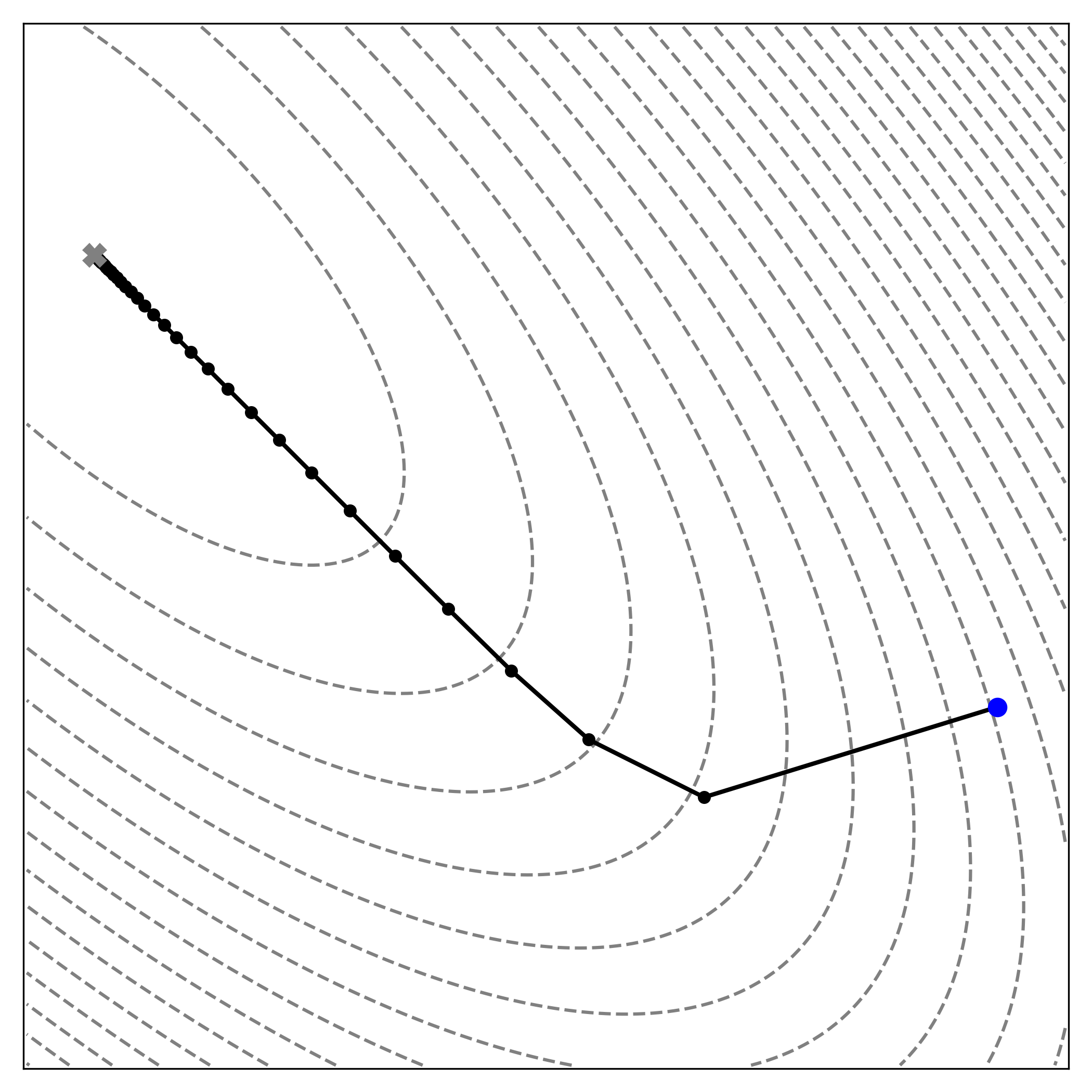 |
| The blue dot indicates the initial point \(\mathbf{x}_0\), and the “x” marks the target (i.e., the minimum). Gradient descent requires 93 steps to reach the minimum in this instance, though the number of iterations depends on the choice of step size \(\alpha\). |
Steepest Descent
While gradient descent requires a manually specified value for \(\alpha\), steepest descent selects the step size at each step \(k\) in a more principled way. Specifically, it chooses the value that minimizes the objective \(f\) along the search direction \(\mathbf{p}_k\):
\[ \begin{equation}\label{eq:sd-alpha} h(\alpha) = f(\mathbf{x}_k + \alpha \mathbf{p}_k) \;. \end{equation} \]
To find the minimizer, we differentiate \(h(\alpha)\) with respect to \(\alpha\) and solve for the point at which the derivative is zero:
\[ \begin{equation*} h(\alpha) = \frac{1}{2} (\mathbf{x}_k + \alpha \mathbf{p}_k)^\top \mathbf{A} (\mathbf{x}_k + \alpha \mathbf{p}_k) - \mathbf{b}^\top (\mathbf{x}_k + \alpha \mathbf{p}_k) + c \;. \end{equation*} \]
Differentiating using the chain rule yields:
\[ \begin{align*} h’(\alpha) &= \frac{d}{d\alpha} f(\mathbf{x}_k + \alpha \mathbf{p}_k) \\ &= \nabla f(\mathbf{x}_k + \alpha \mathbf{p}_k)^\top \frac{d}{d\alpha}(\mathbf{x}_k + \alpha \mathbf{p}_k) \\ &= \nabla f(\mathbf{x}_k + \alpha \mathbf{p}_k)^\top \mathbf{p}_k \\ &= \left[ \mathbf{A}(\mathbf{x}_k + \alpha \mathbf{p}_k) - \mathbf{b} \right]^\top \mathbf{p}_k \\ &= \left[ \mathbf{A} \mathbf{x}_k + \alpha \mathbf{A} \mathbf{p}_k - \mathbf{b} \right]^\top \mathbf{p}_k \\ &= \left[ (\mathbf{A} \mathbf{x}_k - \mathbf{b}) + \alpha \mathbf{A} \mathbf{p}_k \right]^\top \mathbf{p}_k \\ &= (\mathbf{A} \mathbf{x}_k - \mathbf{b})^\top \mathbf{p}_k + \alpha (\mathbf{A} \mathbf{p}_k)^\top \mathbf{p}_k \\ &= -\mathbf{r}_k^\top \mathbf{p}_k + \alpha (\mathbf{A} \mathbf{p}_k)^\top \mathbf{p}_k && \text{by Equation \(\eqref{eq:residual}\)} \\ &= -\mathbf{r}_k^\top \mathbf{p}_k + \alpha \mathbf{p}_k^\top \mathbf{A} \mathbf{p}_k && \text{by the symmetry of \(\mathbf{A}\)} \end{align*} \]
Setting \(h’(\alpha_k) = 0\) and solving for \(\alpha_k\) gives:
\[ \begin{align} -\mathbf{r}_k^\top \mathbf{p}_k + \alpha_k \mathbf{p}_k^\top \mathbf{A} \mathbf{p}_k &= 0 \nonumber \\ \alpha_k &= \frac{\mathbf{r}_k^\top \mathbf{p}_k}{\mathbf{p}_k^\top \mathbf{A} \mathbf{p}_k} \;. \label{eq:step-size} \end{align} \]
The next iterate is then computed using Equation \(\eqref{eq:next-iterate}\).
As previously established, \(f\) has a unique global minimum due to the symmetry and positive definiteness of \(\mathbf{A}\). However, minimizing \(h(\alpha) = f(\mathbf{x}_k + \alpha \mathbf{p}_k)\) only yields the minimum of \(f\) along the line defined by \(\mathbf{p}_k\). Unless \(\mathbf{p}_k\) points directly toward the global minimizer \(\mathbf{x}^*\), the new point \(\mathbf{x}_{k+1}\) will not, in general, be the solution to the original problem. Thus, a new residual is computed using Equation \(\eqref{eq:residual}\) as:
\[ \begin{equation*} \mathbf{r}_{k+1} = \mathbf{b} - \mathbf{A} \mathbf{x}_{k+1} \;. \end{equation*} \]
This expression can be evaluated more efficiently using Equation \(\eqref{eq:next-iterate}\):
\[ \begin{align} \mathbf{r}_{k+1} &= \mathbf{b} - \mathbf{A}(\mathbf{x}_k + \alpha_k \mathbf{p}_k) && \text{by Equation } \eqref{eq:next-iterate} \nonumber \\ &= (\mathbf{b} - \mathbf{A} \mathbf{x}_k) - \alpha_k \mathbf{A} \mathbf{p}_k \nonumber \\ &= \mathbf{r}_k - \alpha_k \mathbf{A} \mathbf{p}_k \;. \label{eq:next-residual} \end{align} \]
This form avoids an additional matrix-vector multiplication by reusing \(\mathbf{A} \mathbf{p}_k\), which was computed when evaluating \(\alpha_k\) in Equation \(\eqref{eq:step-size}\).
The next search direction is set as:
\[ \begin{equation}\label{eq:next-search-direction} \mathbf{p}_{k+1} = \mathbf{r}_{k+1} \;, \end{equation} \]
and the process repeats until convergence.
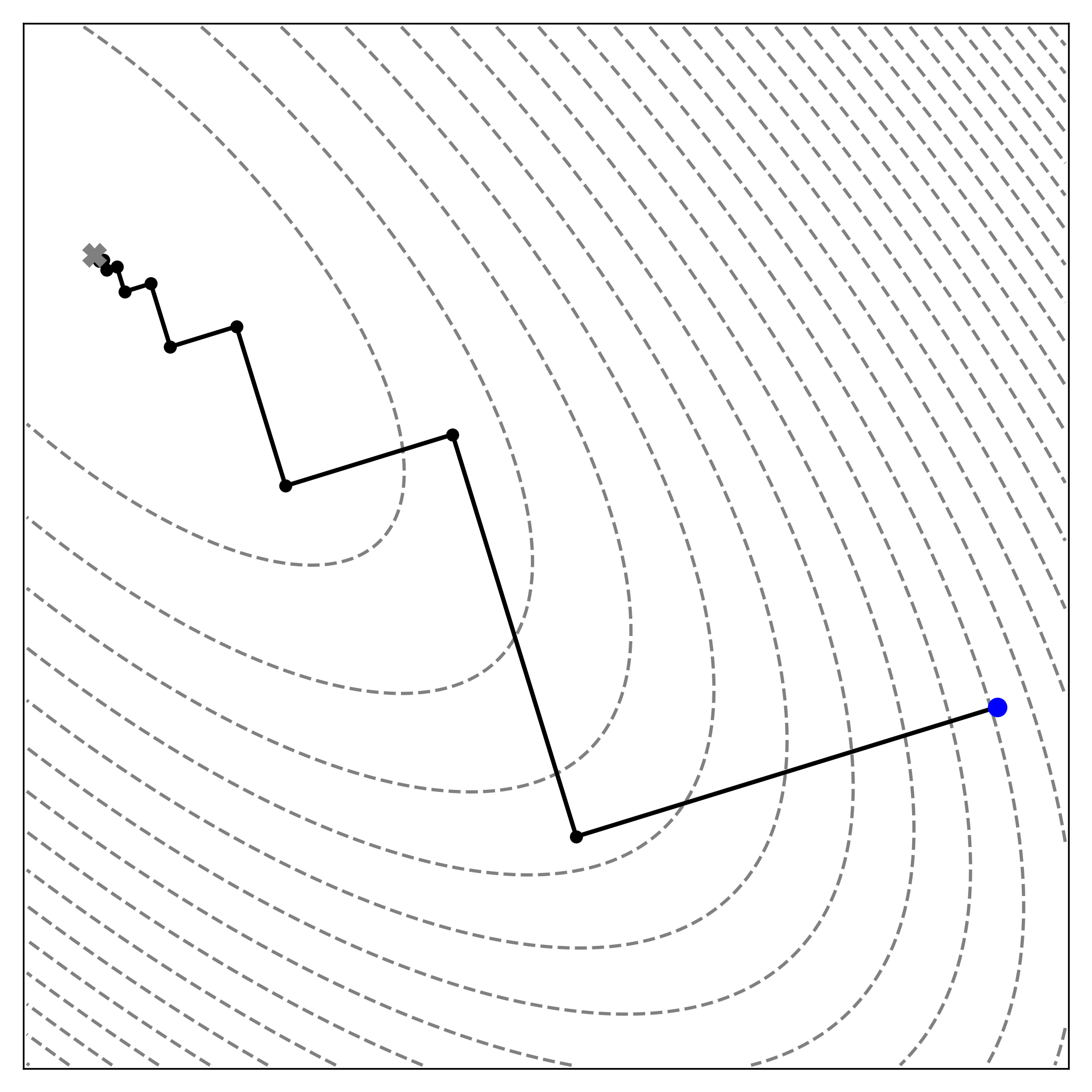 |
| Steepest descent, which chooses \(\alpha_k\) to exactly minimize \(f(\mathbf{x})\) along the negative gradient direction, reaches the minimum in 35 steps. |
Notice in the figure above that each step is orthogonal to the previous step. This is not coincidental, it follows directly from the optimality condition along each search direction. At iteration \(k\), the algorithm moves from \(\mathbf{x}_k\) along the steepest descent direction \(\mathbf{p}_k = -\nabla f(\mathbf{x}_k)\). The line search then selects the point \(\mathbf{x}_{k+1}\) along this direction that minimizes \(f\). Crucially, because \(\mathbf{x}_{k+1}\) minimizes \(f\) along the line defined by \(\mathbf{p}_k\), the instantaneous rate of change of \(f\) at \(\mathbf{x}_{k+1}\) in the direction \(\mathbf{p}_k\) must be zero. If it were not, then continuing in that direction would further decrease the function value, contradicting the definition of \(\mathbf{x}_{k+1}\) as the minimum along that line. This condition is captured by the directional derivative, expressed as the dot product:
\[ \begin{equation}\label{eq:direction-derivative} \nabla f(\mathbf{x}_{k+1}) \cdot \mathbf{p}_k = 0 \;. \end{equation} \]
This equation is precisely the mathematical definition of orthogonality between the gradient vector at the new point, \(\nabla f(\mathbf{x}_{k+1})\), and the previous direction vector \(\mathbf{p}_k\) (assuming neither is the zero vector). Because the next search direction is defined as \(\mathbf{p}_{k+1} = -\nabla f(\mathbf{x}_{k+1})\), this orthogonality is inherited, ensuring that \(\mathbf{p}_{k+1}\) is orthogonal to \(\mathbf{p}_k\).
Because search directions are equal to residuals (Equation \(\eqref{eq:next-search-direction}\)), this orthogonality can be confirmed algebraically by showing that the dot product of consecutive residuals satisfies \(\mathbf{r}_{k+1}^\top \mathbf{r}_k = 0\). Starting from the update rule for the residual:
\[ \begin{align} \mathbf{r}_{k+1}^\top \mathbf{r}_k &= (\mathbf{r}_k - \alpha_k \mathbf{A} \mathbf{p}_k)^\top \mathbf{r}_k && \text{by Equation } \eqref{eq:next-residual} \nonumber \\ &= (\mathbf{r}_k - \alpha_k \mathbf{A} \mathbf{r}_k)^\top \mathbf{r}_k && \text{by Equation } \eqref{eq:next-search-direction} \nonumber \\ &= \left( \mathbf{r}_k^\top - \alpha_k (\mathbf{A} \mathbf{r}_k)^\top \right) \mathbf{r}_k \nonumber \\ &= \left( \mathbf{r}_k^\top - \alpha_k \mathbf{r}_k^\top \mathbf{A}^\top \right) \mathbf{r}_k \nonumber \\ &= \left( \mathbf{r}_k^\top - \alpha_k \mathbf{r}_k^\top \mathbf{A} \right) \mathbf{r}_k && \text{by symmetry of } \mathbf{A} \nonumber \\ &= \mathbf{r}_k^\top \mathbf{r}_k - \alpha_k \mathbf{r}_k^\top \mathbf{A} \mathbf{r}_k \nonumber \\ &= \mathbf{r}_k^\top \mathbf{r}_k - \left( \frac{\mathbf{r}_k^\top \mathbf{p}_k}{\mathbf{p}_k^\top \mathbf{A} \mathbf{p}_k} \right) \mathbf{r}_k^\top \mathbf{A} \mathbf{r}_k && \text{substituting } \alpha_k \text{ from Equation } \eqref{eq:step-size} \nonumber \\ &= \mathbf{r}_k^\top \mathbf{r}_k - \left( \frac{\mathbf{r}_k^\top \mathbf{r}_k}{\mathbf{r}_k^\top \mathbf{A} \mathbf{r}_k} \right) \mathbf{r}_k^\top \mathbf{A} \mathbf{r}_k && \text{since } \mathbf{p}_k = \mathbf{r}_k \nonumber \\ &= \mathbf{r}_k^\top \mathbf{r}_k - \mathbf{r}_k^\top \mathbf{r}_k \nonumber \\ &= 0 \;. \label{eq:orthogonal-residuals} \end{align} \]
This confirms that \(\mathbf{r}_{k+1}\) is orthogonal to \(\mathbf{r}_k\), consistent with the geometric interpretation of steepest descent under exact line search.
The Conjugate Gradient Method
The characteristic zigzagging behavior of steepest descent arises because each new search direction is orthogonal to the previous gradient, but not necessarily well-aligned with the direction of the solution. This inefficiency leads to the method repeatedly “undoing” progress made in earlier steps. The Conjugate Gradient (CG) method, by contrast, chooses search directions that are not merely orthogonal but conjugate — a condition that ensures progress along one direction does not interfere with progress made along others.
Conjugacy
At the \(k\)‑th iteration of any descent method, the error relative to the solution \(\mathbf{x}^*\) can be defined as
\[ \begin{equation}\label{eq:error} \mathbf{e}_k = \mathbf{x}_k - \mathbf{x}^* \;. \end{equation} \]
Ideally, each step of an iterative algorithm should eliminate a distinct component of the error without undoing progress made in earlier steps. In steepest descent, overlapping directions undermine this objective. Conjugacy imposes a geometric structure that prevents reintroduction of error, ensuring that components removed in one step remain eliminated in all subsequent steps.
This principle — that conjugacy prevents the reintroduction of error — can be formalized by examining orthogonality relationships between gradients. By replacing the residuals in Equation \(\eqref{eq:orthogonal-residuals}\) with gradients (justified by Equation \(\eqref{eq:residual-gradient}\)), gives the Euclidean orthogonality condition \(\mathbf{g}_k^\top \mathbf{g}_{k+1}=0\). Substituting \(\mathbf{g}_{k+1}= \mathbf{Ax}_{k+1} - \mathbf{b}\) (by Equation \(\eqref{eq:optimal-x-derived}\)) into that orthogonality relation yields:
\[ \begin{align} 0 &= \mathbf{g}_k^\top \mathbf{g}_{k+1} \nonumber \\ &= \mathbf{g}_k^\top \left( \mathbf{A} \mathbf{x}_{k+1} - \mathbf{b} \right) && \text{by Equation } \nonumber \eqref{eq:optimal-x-derived} \\ &= \mathbf{g}_k^\top \mathbf{A} \left( \mathbf{x}_{k+1} - \mathbf{A}^{-1} \mathbf{b} \right) \nonumber \\ &= \mathbf{g}_k^\top \mathbf{A} \left( \mathbf{x}_{k+1} - \mathbf{x}^* \right) && \text{by Equation } \eqref{eq:closed-from-solution} \nonumber \\ &= \mathbf{g}_k^\top \mathbf{A} \mathbf{e}_{k+1} && \text{by Equation } \eqref{eq:error} \;. \label{eq:orthogonal-error} \end{align} \]
This derivation shows that the new error \(\mathbf{e}_{k+1}\) is orthogonal to the current gradient \(\mathbf{g}_k\) under the \(A\)-inner product:
\[ \begin{equation*} \langle \mathbf{u}, \mathbf{v} \rangle_A = \mathbf{u}^\top \mathbf{A} \mathbf{v} \;. \end{equation*} \]
Orthogonality under this metric, called conjugacy, is the central geometric property underpinning the CG method.
The result in Equation \(\eqref{eq:orthogonal-error}\) motivates constructing the next search direction \(\mathbf{p}_{k+1}\) to align with the new gradient \(\mathbf{g}_{k+1}\) (to reduce remaining error), while being \(A\)-orthogonal to previous search directions \(\mathbf{p}_i\) for \(i \le k\) (to avoid reintroducing eliminated error components). Geometrically, \(\mathbf{p}_{k+1}\) should lie in the span:
\[ \begin{equation*} \mathbf{p}_{k+1} \; \in \; \mathrm{span}\{\mathbf{g}_{k+1}, \mathbf{p}_k\} \;, \end{equation*} \]
with the unique choice satisfying the conjugacy condition:
\[ \begin{equation*} \mathbf{p}_{k+1}^\top \mathbf{A} \mathbf{p}_k = 0 \;. \end{equation*} \]
Here, the span comprises all vectors of the form \(\alpha \mathbf{g}_{k+1} + \beta \mathbf{p}_k\) for scalars \(\alpha, \beta \in \mathbb{R}\).
CG realizes this structure by setting:
\[ \begin{align} \mathbf{p}_0 &= \mathbf{r}_0 \label{eq:initial-direction} \\ \mathbf{p}_{k+1} &= \mathbf{r}_{k+1} + \beta_k \mathbf{p}_k \;, \label{eq:next-direction} \end{align} \]
where the scalar \(\beta_k\) is chosen to enforce \(A\)-orthogonality between consecutive directions. Imposing the conjugacy condition yields:
\[ \begin{align} (\mathbf{r}_{k+1} + \beta_k \mathbf{p}_k)^\top \mathbf{A} \mathbf{p}_k &= 0 \nonumber \\ \mathbf{r}_{k+1}^\top \mathbf{A} \mathbf{p}_k + \beta_k \mathbf{p}_k^\top \mathbf{A} \mathbf{p}_k &= 0 \nonumber \\ \beta_k &= -\frac{\mathbf{r}_{k+1}^\top \mathbf{A} \mathbf{p}_k}{\mathbf{p}_k^\top \mathbf{A} \mathbf{p}_k} \;. \label{eq:beta} \end{align} \]
Computing the step size \(\alpha\)
As in steepest descent (Equation \(\eqref{eq:sd-alpha}\)), the optimal step size \(\alpha_k\) is chosen to minimize the function:
\[ \begin{equation*} h(\alpha) = f(\mathbf{x}_k + \alpha \mathbf{p}_k) \;, \end{equation*} \]
thereby ensuring exact minimization of \(f\) along \(\mathbf{p}_k\) at each iteration. Applying the same derivation that produced Equation \(\eqref{eq:step-size}\), \(\alpha_k\) is computed as:
\[ \begin{equation} \alpha_k = \frac{-\mathbf{g}_k^\top \mathbf{p}_k}{\mathbf{p}_k^\top \mathbf{A} \mathbf{p}_k} \;. \label{eq:optimal-alpha} \end{equation} \]
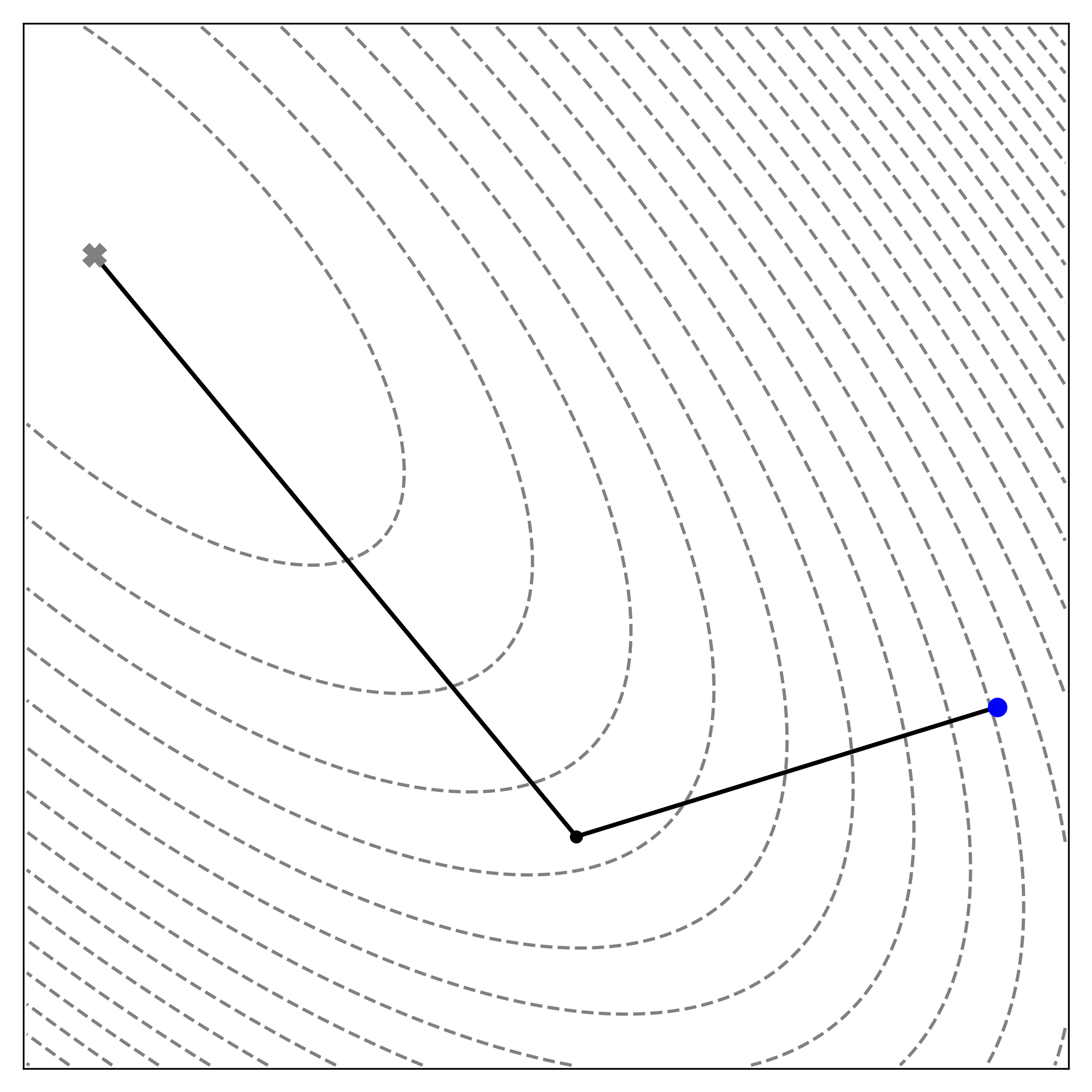 |
| By aligning its search directions with the geometry induced by \(\mathbf{A}\), CG reaches the minimum in just two steps — one per dimension — as each direction eliminates error in a distinct \(A\)-orthogonal component. |
Proving Global Conjugacy by Induction
Having established the procedure for computing \(\mathbf{p}\), \(\alpha\), and \(\beta\), it remains to show that the choice of \(\beta\) in Equation \(\eqref{eq:beta}\) guarantees conjugacy with all preceding directions. We will prove by induction on \(k\), the number of generated directions, that the set \(\{\mathbf{p}_0, \mathbf{p}_1, \dots, \mathbf{p}_{k-1}\}\) is A-conjugate for any \(k \ge 1\).
More formally, let \(P(k)\) denote the statement:
\[ \begin{equation}\label{eq:global-conjugacy-statement} \mathbf{p}_i^\top \mathbf{A} \mathbf{p}_j = 0 \qquad \text{for all } i \ne j, \text{ where } 0 \le i, j < k \;. \end{equation} \]
We will show that \(P(k)\) holds for all \(k \ge 1\). This A-conjugacy ensures that each search direction preserves orthogonality with respect to the \(\mathbf{A}\)-inner product, thereby maintaining the progress of prior steps.
Base Cases
For \(k = 1\), the set \(\{\mathbf{p}_0\}\) contains only one direction, so no distinct indices \(i \ne j\) exist and the condition in Equation \(\eqref{eq:global-conjugacy-statement}\) is vacuously satisfied. Thus, \(P(1)\) holds. For \(k = 2\), \(P(2)\) requires that \(\mathbf{p}_1^\top \mathbf{A} \mathbf{p}_0 = 0\) for the set \(\{\mathbf{p}_0, \mathbf{p}_1\}\). By construction, \(\mathbf{p}_1 = \mathbf{r}_1 + \beta_0 \mathbf{p}_0\) (Equation \(\eqref{eq:next-direction}\)), with \(\beta_0\) chosen to enforce:
\[ \begin{equation*} (\mathbf{r}_1 + \beta_0 \mathbf{p}_0)^\top \mathbf{A} \mathbf{p}_0 = 0 \;, \end{equation*} \]
via Equation \(\eqref{eq:beta}\). It therefore follows directly that \(\mathbf{p}_1^\top \mathbf{A} \mathbf{p}_0 = 0\), confirming \(P(2)\).
Inductive Hypothesis
Assume that \(P(K)\) holds for some integer \(K \ge 1\).
Inductive Step
Assuming the inductive hypothesis \(P(K)\) is true, it remains to show that \(P(K+1)\) also holds. The property \(P(K+1)\) asserts that the set \(\{\mathbf{p}_0, \mathbf{p}_1, \dots, \mathbf{p}_K\}\) is A-conjugate, as defined by Equation \(\eqref{eq:global-conjugacy-statement}\) with \(k=K+1\). The inductive hypothesis ensures that all pairs of distinct vectors in the subset \(\{\mathbf{p}_0, \dots, \mathbf{p}_{K-1}\}\) are A-conjugate. Thus, establishing \(P(K+1)\) reduces to verifying that the newest direction, \(\mathbf{p}_K\), is A-conjugate to each preceding direction \(\mathbf{p}_0, \dots, \mathbf{p}_{K-1}\). Specifically, it must be shown that
\[ \begin{equation*} \mathbf{p}_K^\top \mathbf{A} \mathbf{p}_j = 0 \quad \text{for all} \quad 0 \le j < K \;. \end{equation*} \]
A-conjugacy with the most recent direction, \(\mathbf{p}_{K-1}\), follows directly from the definition \(\mathbf{p}_K = \mathbf{r}_K + \beta_{K-1} \mathbf{p}_{K-1}\), where \(\beta_{K-1}\) is chosen to enforce \(\mathbf{p}_K^\top \mathbf{A} \mathbf{p}_{K-1} = 0\) (Equation \(\eqref{eq:beta}\)). This mirrors the verification in \(P(2)\).
Next, A-conjugacy for \(\mathbf{p}_K\) with respect to all earlier directions \(\mathbf{p}_j\), where \(j < K-1\), must be established. Expanding \(\mathbf{p}_K = \mathbf{r}_K + \beta_{K-1} \mathbf{p}_{K-1}\) gives
\[ \begin{align*} \mathbf{p}_K^\top \mathbf{A} \mathbf{p}_j &= (\mathbf{r}_K + \beta_{K-1} \mathbf{p}_{K-1})^\top \mathbf{A} \mathbf{p}_j \\ &= \color{blue}{\mathbf{r}_K^\top \mathbf{A} \mathbf{p}_j} + \color{red}{\beta_{K-1} (\mathbf{p}_{K-1}^\top \mathbf{A} \mathbf{p}_j)} \;. \end{align*} \]
Because \(j < K-1\), the directions \(\mathbf{p}_{K-1}\) and \(\mathbf{p}_j\) are distinct elements of \(\{\mathbf{p}_0, \dots, \mathbf{p}_{K-1}\}\). By the inductive hypothesis \(P(K)\), this set is A-conjugate, so \(\mathbf{p}_{K-1}^\top \mathbf{A} \mathbf{p}_j = 0\) and the red term \(\color{red}{\beta_{K-1} (\mathbf{p}_{K-1}^\top \mathbf{A} \mathbf{p}_j)}\) vanishes.
Demonstrating A-conjugacy with all prior directions thus simplifies to proving that the blue term, \(\color{blue}{\mathbf{r}_K^\top \mathbf{A} \mathbf{p}_j}\), is zero. To evaluate this term, an explicit expression for \(\mathbf{A}\mathbf{p}_j\) is required. Rearranging the residual update \(\mathbf{r}_{j+1} = \mathbf{r}_j - \alpha_j \mathbf{A} \mathbf{p}_j\) (Equation \(\eqref{eq:next-residual}\)) yields:
\[ \begin{equation*} \mathbf{A} \mathbf{p}_j = \frac{1}{\alpha_j}(\mathbf{r}_j - \mathbf{r}_{j+1}) \;. \end{equation*} \]
Substituting into \(\color{blue}{\mathbf{r}_K^\top \mathbf{A} \mathbf{p}_j}\) gives
\[ \begin{align} \mathbf{r}_K^\top \mathbf{A} \mathbf{p}_j &= \mathbf{r}_K^\top \left( \frac{1}{\alpha_j}(\mathbf{r}_j - \mathbf{r}_{j+1}) \right) \nonumber \\ &= \frac{1}{\alpha_j} (\mathbf{r}_K^\top \mathbf{r}_j - \mathbf{r}_K^\top \mathbf{r}_{j+1}) \;. \label{eq:inductive-task} \end{align} \]
This expression is zero if the current residual \(\mathbf{r}_K\) is orthogonal to all previous residuals; that is, if \(\mathbf{r}_K^\top \mathbf{r}_j = 0\) and \(\mathbf{r}_K^\top \mathbf{r}_{j+1} = 0\). It therefore remains to establish the general property \(\mathbf{r}_K^\top \mathbf{r}_m = 0\) for all \(m < K\).
To demonstrate residual orthogonality, \(\mathbf{r}_K^\top \mathbf{r}_m = 0\) for \(m < K\), first note that any previous residual \(\mathbf{r}_m\) can be written as a linear combination of the search directions up to \(\mathbf{p}_m\). Specifically, for the base case \(m = 0\), Equation \(\eqref{eq:initial-direction}\) gives \(\mathbf{p}_0 = \mathbf{r}_0\), so \(\mathbf{r}_0 = 1 \cdot \mathbf{p}_0\), and thus \(\mathbf{r}_0 \in \mathrm{span}\{\mathbf{p}_0\}\). For \(m > 0\), Equation \(\eqref{eq:next-direction}\) gives:
\[ \begin{align*} \mathbf{p}_m &= \mathbf{r}_m + \beta_{m-1} \mathbf{p}_{m-1} \\ \mathbf{r}_m &= \mathbf{p}_m - \beta_{m-1} \mathbf{p}_{m-1} \;. \end{align*} \]
Because \(\mathbf{p}_m, \mathbf{p}_{m-1} \in \{\mathbf{p}_0, \dots, \mathbf{p}_m\}\), it follows that \(\mathbf{r}_m\) can be written as a linear combination of all vectors in \(\{\mathbf{p}_0, \dots, \mathbf{p}_m\}\) by assigning zero coefficients to all vectors other than \(\mathbf{p}_m\) and \(\mathbf{p}_{m-1}\):
\[ \begin{equation*} \mathbf{r}_m = \sum_{i=0}^{m} c_i \mathbf{p}_i \;, \end{equation*} \]
for some coefficients \(c_i\).
The inner product \(\mathbf{r}_K^\top \mathbf{r}_m\) for \(m < K\) can thus be written as:
\[ \begin{equation}\label{eq:residual-sum} \mathbf{r}_K^\top \mathbf{r}_m = \mathbf{r}_K^\top \left( \sum_{i=0}^{m} c_i \mathbf{p}_i \right) = \sum_{i=0}^{m} c_i (\mathbf{r}_K^\top \mathbf{p}_i) \;. \end{equation} \]
This sum is zero if \(\mathbf{r}_K^\top \mathbf{p}_i = 0\) for all \(i \le m < K\). It is therefore necessary to show that the current residual \(\mathbf{r}_K\) is orthogonal to all previous search directions \(\mathbf{p}_i\) for \(i < K\).
To prove \(\mathbf{r}_K^\top \mathbf{p}_i = 0\) for \(i < K\), consider two cases for the index \(i\). For \(i = K-1\), the orthogonality \(\mathbf{r}_K^\top \mathbf{p}_{K-1} = 0\) follows from the exact line search at iteration \(K-1\), which ensures the gradient at \(\mathbf{x}_K\) is orthogonal to the search direction \(\mathbf{p}_{K-1}\). Specifically, for the step from \(\mathbf{x}_{K-1}\) to \(\mathbf{x}_K\) along \(\mathbf{p}_{K-1}\),
\[ \begin{align*} \nabla f(\mathbf{x}_K)^\top \mathbf{p}_{K-1} &= 0 && \text{by Equation } \eqref{eq:direction-derivative} \\ \mathbf{g}_K^\top \mathbf{p}_{K-1} &= 0 && \text{where } \mathbf{g}_K = \nabla f(\mathbf{x}_K) \\ \mathbf{r}_K^\top \mathbf{p}_{K-1} &= 0 && \text{by Equation } \eqref{eq:residual-gradient} \text{ (since } \mathbf{r}_K = -\mathbf{g}_K \text{)}\;. \end{align*} \]
Thus, \(\mathbf{r}_K\) is orthogonal to the most recent prior direction \(\mathbf{p}_{K-1}\).
For the earlier directions (\(i < K-1\)), we rely on gradient recurrence. Because \(\mathbf{r}_m = -\mathbf{g}_m\), the residual update \(\mathbf{r}_{m+1} = \mathbf{r}_m - \alpha_m \mathbf{A}\mathbf{p}_m\) (Equation \(\eqref{eq:next-residual}\)) yields:
\[ \begin{equation*} \mathbf{g}_K = \mathbf{g}_{K-1} + \alpha_{K-1} \mathbf{A} \mathbf{p}_{K-1} \;. \end{equation*} \]
Taking the inner product with \(\mathbf{p}_i\) for \(i < K-1\) gives:
\[ \begin{align*} \mathbf{g}_K^\top \mathbf{p}_i &= (\mathbf{g}_{K-1} + \alpha_{K-1} \mathbf{A} \mathbf{p}_{K-1})^\top \mathbf{p}_i \\ &= \mathbf{g}_{K-1}^\top \mathbf{p}_i + \alpha_{K-1} (\color{red}{\mathbf{p}_{K-1}^\top \mathbf{A} \mathbf{p}_i}) \;. \end{align*} \]
By the inductive hypothesis \(P(K)\) (Equation \(\eqref{eq:global-conjugacy-statement}\)), the term \(\color{red}{\mathbf{p}_{K-1}^\top \mathbf{A} \mathbf{p}_i} = 0\) for \(i < K-1\). Thus, the recurrence reduces to \(\mathbf{g}_K^\top \mathbf{p}_i = \mathbf{g}_{K-1}^\top \mathbf{p}_i\). Repeatedly applying this relationship gives:
\[ \begin{equation*} \mathbf{g}_K^\top \mathbf{p}_i = \mathbf{g}_{K-1}^\top \mathbf{p}_i = \dots = \color{blue}{\mathbf{g}_{i+1}^\top \mathbf{p}_i} \;. \end{equation*} \]
The final term, \(\color{blue}{\mathbf{g}_{i+1}^\top \mathbf{p}_i}\), vanishes due to the exact line search at iteration \(i\), which ensures \(\nabla f(\mathbf{x}_{i+1})\) is orthogonal to \(\mathbf{p}_i\) (Equation \(\eqref{eq:direction-derivative}\)).
Combining both cases (\(i = K-1\) and \(i < K-1\)), it is now established that the current residual is orthogonal to all previous search directions:
\[ \begin{equation}\label{eq:residual-direction-orthogonality-established-final} \mathbf{r}_K^\top \mathbf{p}_i = 0 \quad \text{for all } i < K \;. \end{equation} \]
Returning to Equation \(\eqref{eq:residual-sum}\), since \(i \le m < K\), Equation \(\eqref{eq:residual-direction-orthogonality-established-final}\) guarantees that each term \(\mathbf{r}_K^\top \mathbf{p}_i\) in the sum is zero. Thus, the entire sum vanishes, establishing the orthogonality of residuals:
\[ \begin{equation}\label{eq:residual-orthogonality-established-final} \mathbf{r}_K^\top \mathbf{r}_m = 0 \quad \text{for all } m < K \;. \end{equation} \]
With this crucial result, Equation \(\eqref{eq:inductive-task}\) can finally be evaluated:
\[ \begin{equation*} \mathbf{r}_K^\top \mathbf{A} \mathbf{p}_j = \frac{1}{\alpha_j} (\mathbf{r}_K^\top \mathbf{r}_j - \mathbf{r}_K^\top \mathbf{r}_{j+1}) \;. \end{equation*} \]
Because \(j < K-1\), it must be true that \(j < K\) and \(j+1 < K\). By the established residual orthogonality (Equation \(\eqref{eq:residual-orthogonality-established-final}\)), \(\mathbf{r}_K^\top \mathbf{r}_j = 0\) and \(\mathbf{r}_K^\top \mathbf{r}_{j+1} = 0\), so \(\mathbf{r}_K^\top \mathbf{A} \mathbf{p}_j = 0\). Thus, the first term in the expression for \(\mathbf{p}_K^\top \mathbf{A} \mathbf{p}_j\) vanishes, and for \(j < K-1\), \(\mathbf{p}_K^\top \mathbf{A} \mathbf{p}_j = 0\).
Given \(\mathbf{p}_K^\top \mathbf{A} \mathbf{p}_j = 0\) has been shown for both \(j = K-1\) and all \(j < K-1\), it follows that \(\mathbf{p}_K\) is A-conjugate to all preceding directions \(\mathbf{p}_0, \dots, \mathbf{p}_{K-1}\). Therefore, \(P(K+1)\) holds.
Practical implementation
The expression for \(\alpha_k\) in Equation \(\eqref{eq:optimal-alpha}\) involves the inner product between the gradient \(\mathbf{g}_k\) and the search direction \(\mathbf{p}_k\):
\[ \begin{equation*} \alpha_k = \frac{-\mathbf{g}_k^\top \mathbf{p}_k}{\mathbf{p}_k^\top \mathbf{A} \mathbf{p}_k} \;. \end{equation*} \]
This computation can be simplified by rewriting the numerator. First, observe that:
\[ \begin{align*} -\mathbf{g}_k^\top \mathbf{p}_k &= \mathbf{r}_k^\top \mathbf{p}_k && \text{by definition of the residual} \\ &= \mathbf{r}_k^\top (\mathbf{r}_k + \beta_{k-1} \mathbf{p}_{k-1}) && \text{by Equation } \eqref{eq:next-direction} \\ &= \mathbf{r}_k^\top \mathbf{r}_k + \beta_{k-1} \mathbf{r}_k^\top \mathbf{p}_{k-1} \\ &= \mathbf{r}_k^\top \mathbf{r}_k && \text{since } \mathbf{r}_k^\top \mathbf{p}_{k-1} = 0 \text{ by Equation } \eqref{eq:residual-direction-orthogonality-established-final} \end{align*} \]
Substituting this into Equation \(\eqref{eq:optimal-alpha}\) yields the simplified expression:
\[ \begin{equation}\label{eq:simplified-alpha} \alpha_k = \frac{\mathbf{r}_k^\top \mathbf{r}_k}{\mathbf{p}_k^\top \mathbf{A} \mathbf{p}_k} \;. \end{equation} \]
This form is preferred in practice, as the numerator \(\mathbf{r}_k^\top \mathbf{r}_k\) is already computed during the update for \(\beta_k\) and can be reused. More specifically, the expression for \(\beta_k\) in Equation \(\eqref{eq:beta}\) can be similarly simplified using the residual update formula \(\mathbf{r}_{k+1} = \mathbf{r}_k - \alpha_k \mathbf{A} \mathbf{p}_k\) (Equation \(\eqref{eq:next-residual}\)) via Equation \(\eqref{eq:inductive-task}\) and the orthogonality property \(\mathbf{r}_{k+1}^\top \mathbf{r}_k = 0\) (Equation \(\eqref{eq:residual-orthogonality-established-final}\)):
\[ \begin{align*} \beta_k &= -\frac{\mathbf{r}_{k+1}^\top \mathbf{A} \mathbf{p}_k}{\mathbf{p}_k^\top \mathbf{A} \mathbf{p}_k} \\ &= - \frac{\mathbf{r}_{k+1}^\top (\mathbf{r}_k - \mathbf{r}_{k+1}) / \alpha_k}{\mathbf{p}_k^\top \mathbf{A} \mathbf{p}_k} && \text{by Equation } \eqref{eq:inductive-task} \\ &= - \frac{\mathbf{r}_{k+1}^\top \mathbf{r}_k / \alpha_k - \mathbf{r}_{k+1}^\top \mathbf{r}_{k+1} / \alpha_k}{\mathbf{p}_k^\top \mathbf{A} \mathbf{p}_k} \\ &= \frac{\mathbf{r}_{k+1}^\top \mathbf{r}_{k+1} / \alpha_k}{\mathbf{p}_k^\top \mathbf{A} \mathbf{p}_k} && \text{by Equation } \eqref{eq:residual-orthogonality-established-final} \\ &= \frac{\mathbf{r}_{k+1}^\top \mathbf{r}_{k+1} / \left(\frac{\mathbf{r}_k^\top \mathbf{r}_k}{\mathbf{p}_k^\top \mathbf{A} \mathbf{p}_k} \right)}{\mathbf{p}_k^\top \mathbf{A} \mathbf{p}_k} && \text{by Equation } \eqref{eq:simplified-alpha} \\ &= \frac{\mathbf{r}_{k+1}^\top \mathbf{r}_{k+1} \cdot \mathbf{p}_k^\top \mathbf{A} \mathbf{p}_k}{\mathbf{r}_k^\top \mathbf{r}_k \cdot \mathbf{p}_k^\top \mathbf{A} \mathbf{p}_k} \\ &= \frac{\mathbf{r}_{k+1}^\top \mathbf{r}_{k+1}}{\mathbf{r}_k^\top \mathbf{r}_k} \;. \end{align*} \]
This final form is computationally efficient: it requires only inner products of residuals, avoiding any additional matrix-vector multiplications.
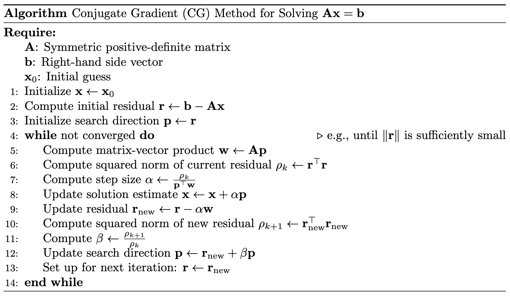
In summary, CG proceeds by first moving in the direction of steepest descent (\(\mathbf{p}_0 = \mathbf{r}_0\)). At each iteration \(k\), it selects a step size \(\alpha_k\) to exactly minimize the objective along the current search direction \(\mathbf{p}_k\). The new residual \(\mathbf{r}_{k+1}\) is then computed using the previous residual and the matrix-vector product \(\mathbf{A}\mathbf{p}_k\). A new search direction \(\mathbf{p}_{k+1}\) is formed by combining the new residual \(\mathbf{r}_{k+1}\) with a scaled contribution from \(\mathbf{p}_k\), where the scaling factor \(\beta_k\) is chosen to ensure \(A\)-conjugacy between \(\mathbf{p}_{k+1}\) and \(\mathbf{p}_k\). This construction recursively maintains \(A\)-conjugacy with all previous directions. Global \(A\)-conjugacy ensures that the search directions are independent relative to the geometry induced by \(\mathbf{A}\), allowing the algorithm to eliminate error components sequentially without interference, thereby minimizing the objective (Equation \(\eqref{eq:quadratic}\)) efficiently.
 |
Citation
Landers, Matthew. "Conjugate Gradient Method." mattlanders.net, May 26, 2025. mattlanders.net/conjugate-gradient-method.
@article{landers2025conjugate,
  title = {Conjugate Gradient Method},
  author = {Landers, Matthew},
  journal = {mattlanders.net},
  year = {2025},
  month = {May},
  url = "mattlanders.net/conjugate-gradient-method"
}
References
- An Introduction to the Conjugate Gradient Method Without the Agonizing Pain (1994)
Jonathan Richard Shewchuk
- Conjugate Gradient Descent (2022)
Gregory Gundersen
- Understanding Positive Definite Matrices (2022)
Gregory Gundersen