Off-Policy Control with Function Approximation

While SARSA and Q-learning share fundamental principles, off-policy methods present two challenges absent in on-policy learning. The first emerges in both tabular and function approximation settings and has a straightforward solution. The second challenge, specific to the use of function approximation, requires separate theoretical treatments for on- and off-policy learning. This note focuses exclusively on off-policy learning; the corresponding discussion of on-policy learning is presented in a dedicated note.

The first challenge in off-policy learning arises from the use of samples generated by a behavior policy \(\pi_\beta\) to learn the value function with respect to a target policy \(\pi\). To accurately update the value function, off-policy methods must account for the discrepancy between \(\pi_\beta\) and \(\pi\). The importance sampling ratio \(\rho_t = \frac{\pi(a_t \mid s_t)}{\pi_\beta(a_t \mid s_t)}\) provides the necessary correction. For example, the off-policy analog of the one-step on-policy semi-gradient TD(0) update takes the following form:

\[ \begin{align} \theta_{t+1} &= \theta_t + \alpha \rho_t \left[ r_{t+1} + \gamma \hat{V}(s_{t+1}; \theta_t) - \hat{V}(s_t; \theta_t) \right] \nabla \hat{V}(s_t; \theta_t) \label{eq:off-policy-td-update-1} \\ &= \theta_t + \alpha \rho_t \delta_t \nabla \hat{V}(s_t; \theta_t) \;. \nonumber \end{align} \]

The second challenge, unique to function approximation in off-policy learning, is notably more difficult. The semi-gradient update changes the value estimate at state \(s_t\), which in turn affects the values of subsequent states. In on-policy learning, the state distribution in the training data matches the on-policy distribution \(\mu_\pi\), so updates, on average, adjust the value function in the correct direction for the objective.

In off-policy learning, the update at \(s_t\) is applied to a state sampled from the behavior policy's distribution, \(\mu_\beta\). This introduces a fundamental distributional mismatch — the algorithm minimizes error on states frequent under \(\mu_\beta\), which may not correspond to those most relevant under the target policy \(\pi\). An update that reduces the error at one state can increase it elsewhere, and if states critical to \(\pi\) are rarely sampled, these errors can accumulate and cause divergence.

Although importance sampling appears to be a natural solution, weighting the one-step update by \(\rho_t\) (as in Equation \(\eqref{eq:off-policy-td-update-1}\)) does not resolve the distributional mismatch (see the Deadly Triad note). Ensuring stability requires more advanced methods. Alternatively, true gradient methods can be developed, which remain stable without relying on a specific data distribution. In the remainder of this note, we focus on the use of true gradient methods.

Why Q-learning Does Not use Importance Sampling

The first challenge in off-policy learning — the use of samples generated by a behavior policy \(\pi_\beta\) to estimate the value function for a target policy \(\pi\) — arises in both tabular and approximate settings. The absence of importance sampling in Q-learning thus requires an explanation.

We begin by examining how the target policy influences the Q-learning update:

\[ \begin{equation}\label{eq:q-update} \hat{Q}(s_t, a_t) \gets \hat{Q}(s_t, a_t) + \alpha \left( r_{t+1} + \gamma \color{red}{\max_{a_{t+1}} \hat{Q}(s_{t+1}, a_{t+1})} - \hat{Q}(s_t, a_t) \right) \;. \end{equation} \]

In this update, the target policy is reflected in the \(\max_{a_{t+1}} \hat{Q}(s_{t+1}, a_{t+1})\) term, highlighted in red. This becomes clearer when considering the definition of the Q-value function for an arbitrary policy \(\pi\):

\[ \begin{equation}\label{eq:q-definition} Q_\pi (s, a) = R(s, a) + \gamma \sum_{s’ \in \mathcal{S}} P(s, a, s’) \left( \color{blue}{\sum_{a’ \in \mathcal{A}} \pi(a’ \mid s’) Q_\pi (s’, a’)} \right) \;. \end{equation} \]

Q-learning uses a maximization in Equation \(\eqref{eq:q-update}\) because it approximates the target policy — the optimal policy — directly. This optimal policy is the greedy policy with respect to the optimal action-value function:

\[ \begin{equation}\label{greedy-selection} Q_* (s, a) = R(s, a) + \gamma \sum_{s’ \in \mathcal{S}} P(s, a, s’) \color{red}{\max_{a’} Q_* (s’, a’)} \;, \end{equation} \]

By replacing the expectation over possible actions (the blue term in Equation \(\eqref{eq:q-definition}\)) with the greedy action (the red term in Equation \(\eqref{eq:q-update}\)), the update includes the action that the target (optimal) policy would select (as demonstrated in Equation \(\eqref{greedy-selection}\)). In effect, the behavior policy's action probabilities become irrelevant to the computation, thereby obviating the need for importance sampling.

The utility of importance sampling becomes evident when the update rule relies on an expectation over actions under the target policy \(\pi\) as in Equation \(\eqref{eq:q-definition}\), rather than on the greedy action as in Equation \(\eqref{eq:q-update}\):

\[ \begin{equation*} \hat{Q}(s_t, a_t) \gets \hat{Q}(s_t, a_t) + \alpha \left( r_{t+1} + \gamma \left( \color{blue}{\sum_{a’ \in \mathcal{A}} \pi(a’ \mid s_{t+1}) \hat{Q}(s_{t+1}, a’)} \right) - \hat{Q}(s_t, a_t) \right) \;. \end{equation*} \]

Because samples are generated using \(\pi_\beta\), this expectation becomes biased toward actions favored by the behavior policy. Importance sampling corrects this bias by re-weighting actions according to the ratio of target and behavior policy probabilities, yielding an unbiased estimate of the target policy's value.

Function Approximation Objective

When a policy's true value function \(V_\pi\) is too complex to represent exactly, we approximate it with a parameterized function \(\hat{V}(\theta)\). To find the best approximation of \(V_\pi\), we iteratively adjust the parameters \(\theta\) to minimize a chosen error criterion, measured using a norm. For example, in prediction with function approximation, we often minimize the mean squared error between \(V_\pi\) and \(\hat{V}(\theta)\). This error is quantified using a weighted version of the standard Euclidean norm:

\[ \begin{equation} \| f \|_\mu^2 = \sum_{s \in \mathcal{S}} \mu(s) f(s)^2 \;, \label{eq:squared-norm-of-vector} \end{equation} \]

This norm expresses the magnitude or “length” of a function \(f\) when weighted by the state distribution \(\mu\). Using this norm, we can measure the distance between functions. For instance, the mean squared value error can be represented as \(\overline{\text{VE}} = \| \hat{V}(\theta) - V_\pi \|_\mu^2\), providing a meaningful way to quantify the discrepancy between \(\hat{V}(\theta)\) and the true value function \(V_\pi\).

The Bellman Error

While value error is an appropriate criterion for approximate Monte Carlo (MC) methods — which asymptotically converge to an estimate \(\hat{V}\) that approximates \(V_\pi\) (albeit slowly) — this objective is unsuitable for Temporal Difference (TD) methods due to their use of bootstrapping. Specifically, in MC methods, the update target \(Y_t = G_t\) provides an unbiased estimate of \(V\) because \(\mathbb{E}[G_t \mid s_t = s] = V_\pi(s) \; \forall t\). TD methods, by contrast, use an update target \(Y_t = r_{t+1} + \gamma \hat{V}(s_{t+1}; \theta_t)\), which depends on \(\theta_t\) and is thus a “moving target.” That is, when \(\theta\) is updated to reduce the error between \(Y_t\) and \(\hat{V}\), this change also affects the target value itself, introducing bias into the estimate. Because convergence to a local optimum is guaranteed only when using an unbiased estimator, TD methods instead minimize an objective for which their target is an unbiased estimate of the function being approximated — the mean squared Bellman error.

\[ \begin{equation*} V_\pi (s) = \sum_{a \in \mathcal{A}} \pi(a \mid s) \left( R(s,a) + \gamma \sum_{s’ \in \mathcal{S}} P(s,a,s’) V_\pi (s’) \right) \;. \end{equation*} \]

As demonstrated in the DP for MDPs proofs note, the true value function is the unique fixed point of the Bellman operator, \(\mathcal{T}_\pi\) (this operator is discussed in greater detail in the same note). A fixed point of a transformation \(f\) is defined as a point \(p\) such that \(f(p) = p\). Intuitively, the true value function \(V_\pi\) is the only function that remains unchanged when the Bellman operator is applied. That is, applying \(\mathcal{T}_\pi\) to \(V_\pi\) yields \(V_\pi\) itself.

To quantify deviations from this fixed point, we define the Bellman error as the difference between the current estimate and its update under the Bellman operator. Mathematically, the Bellman error is given by:

\[ \begin{align} \overline{\delta}_{\theta}(s) &= [\mathcal{T}_\pi\hat{V}(\theta)](s) - \hat{V}(s; \theta) \label{eq:bellman-error-1} \\ &= \sum_{a \in \mathcal{A}} \pi(a \mid s) \left[ R(s,a) + \gamma \sum_{s’ \in \mathcal{S}} P(s,a,s’) \hat{V}(s’; \theta) \right] - \hat{V}(s; \theta) \label{eq:bellman-error-2} \\ &= \mathbb{E}_\pi \left[ r_{t+1} + \gamma \hat{V}(s_{t+1}; \theta) - \hat{V}(s_t; \theta) \mid s_t = s \right] \;. \label{eq:bellman-error-3} \end{align} \]

This error measures how well \(\hat{V}(\theta)\) approximates the true value function \(V_\pi\) for a given policy \(\pi\), incorporating an expectation over all possible next states \(s'\), weighted by the transition probabilities \(P(s, a, s’)\). Because the Bellman error is defined over an expectation of all possible transitions, computing it requires knowledge of \(P(s, a, s’)\) (Equation \(\eqref{eq:bellman-error-2}\)). Because \(P(s, a, s’)\) is typically unknown in practice, we cannot compute the Bellman error exactly. Instead, we estimate it by drawing samples from the environment (Equation \(\eqref{eq:bellman-error-3}\)). By sampling multiple transitions starting from state \(s\) and following policy \(\pi\), we can compute the average error over these samples, yielding an unbiased estimate of the Bellman error.

TD error vs. Bellman error

The Bellman error is a theoretical construct closely related to the more practical temporal difference (TD) error. The TD error is a stochastic quantity computed from a single sampled transition \((s_t, a_t, r_{t+1}, s_{t+1})\), defined as

\[ \begin{equation*} \delta_t = r_{t+1} + \gamma \hat{V}(s_{t+1}; \theta) - \hat{V}(s_t; \theta) \;. \end{equation*} \]

Since the next state \(s_{t+1}\) and reward \(r_{t+1}\) are random variables, the TD error \(\delta_t\) is also random.

The Bellman error (Equation \(\eqref{eq:bellman-error-3}\)), is the expectation of the TD error at a given state \(s\). Formally:

\[ \begin{equation*} \overline{\delta}_{\theta}(s) = \mathbb{E}_\pi \left[ \delta_t \mid s_t = s \right] \;. \end{equation*} \]

This expectation is taken over the policy's action distribution and the environment's transition dynamics. Thus, the Bellman error at state \(s\) corresponds to the average TD error over all possible next states and rewards reachable from \(s\).

The relationship between TD error and Bellman error can be summarized as follows: The TD error is a stochastic, sample-based estimate of the Bellman error. It is computationally efficient, requiring only a single transition, but exhibits high variance. The Bellman error is the true expected error at a state. It is deterministic with zero variance. While it could, in principle, be approximated by generating many transitions from the same state \(s\) and averaging the resulting TD errors:

\[ \begin{equation*} \overline{\delta}_{\theta}(s) \approx \frac{1}{N} \sum_{i=1}^{N} \left[ r_{t+1}^{(i)} + \gamma \hat{V}(s_{t+1}^{(i)}; \theta) - \hat{V}(s; \theta) \right] \;, \end{equation*} \]

this approach is impractical in most RL settings as it would require repeatedly resetting the environment to state \(s\) to obtain a sufficient number of samples for each update.

From Equations \(\eqref{eq:squared-norm-of-vector}\) and \(\eqref{eq:bellman-error-1}\), we define the mean squared Bellman error as:

\[ \begin{equation*} \overline{\text{BE}} = \| \overline{\delta}_{\theta} \|_\mu^2 \;. \end{equation*} \]

In general, it is not possible to reduce \(\overline{\text{BE}}\) to zero — where \(\hat{V}(\theta) = V_\pi\) — but for linear function approximation, there exists a unique value of \(\theta\) that minimizes \(\overline{\text{BE}}\). This point is typically different than the point at which \(\overline{\text{VE}}\) is minimized.

Gradient Descent in the Bellman Error

Minimizing the Bellman error is, ostensibly, a reasonable objective. However, this approach is fraught with challenges that warrant careful examination. To establish a foundation for this analysis, we first examine the related problem of minimizing the TD error, as the Bellman error is defined as the expectation of the TD error.

The mean squared TD error is defined as the weighted mean of the squared TD error, with weights corresponding to the frequency of state visits. Mathematically, it is given by:

\[ \begin{align} \overline{\text{TDE}}(\theta) &= \sum_{s \in \mathcal{S}} \mu(s) \mathbb{E}[\delta_t^2 \mid s_t = s, a_t \sim \pi] \label{eq:sgd-td-loss-1} \\ &= \sum_{s \in \mathcal{S}} \mu(s) \mathbb{E}[\rho_t \delta_t^2 \mid s_t = s, a_t \sim \pi_\beta] \nonumber \\ &= \mathbb{E}_{\pi_\beta} [\rho_t \delta_t^2] \;, \label{eq:sgd-td-loss-2} \end{align} \]

where \(\mu\) is the distribution under \(\pi_\beta\), \(\delta_t = r_{t+1} + \gamma \hat{V}(s_{t+1}; \theta_t) - \hat{V}(s_t; \theta_t)\) is the one-step TD error with discounting, and \(\rho_t\) is the importance sampling ratio.

Equation \(\eqref{eq:sgd-td-loss-2}\) expresses the objective as an expectation over samples generated by the behavior policy \(\pi_\beta\). This representation allows unbiased gradient estimation from individual transitions, satisfying a fundamental requirement for stochastic gradient descent (SGD). Specifically, the expectation \(\mathbb{E}_{\pi_\beta}[\rho_t \delta_t^2]\) can be estimated using single transitions \((s, a, r, s’)\) collected under \(\pi_\beta\). For each transition, the TD error \(\delta_t\) and the importance sampling ratio \(\rho_t\) are computed. Their product, \(\rho_t \delta_t^2\), provides an unbiased estimate of the objective function. This unbiasedness follows directly from the definition of an unbiased estimator and is explicitly reflected in Equation \(\eqref{eq:sgd-td-loss-2}\). This contrasts with Equation \(\eqref{eq:sgd-td-loss-1}\), which requires enumerating the entire state space and sampling actions from the target policy \(\pi\) — operations typically infeasible in practice.

Having defined the mean squared TD error objective as an expectation that can be sampled from the experience of the behavior policy \(\pi_\beta\) in Equation \(\eqref{eq:sgd-td-loss-2}\), we now derive the corresponding update rule:

\[ \begin{align} \theta_{t+1} &= \theta_t - \frac{1}{2} \alpha \nabla(\rho_t \delta_t^2) \nonumber \\ &= \theta_t - \frac{1}{2} \alpha \rho_t \nabla(\delta_t^2) && \text{because } \rho_t \text{ is a constant} \nonumber \\ &= \theta_t - \frac{1}{2} \alpha \rho_t \nabla(\delta_t \cdot \delta_t) \nonumber \\ &= \theta_t - \frac{1}{2} \alpha \rho_t \left( (\delta_t \cdot \nabla \delta_t) + (\delta_t \cdot \nabla \delta_t) \right) && \text{by the product rule} \nonumber \\ &= \theta_t - \frac{1}{2} \alpha \rho_t 2(\delta_t \cdot \nabla \delta_t) \nonumber \\ &= \theta_t - \alpha \rho_t \delta_t \nabla \delta_t \nonumber \\ &= \theta_t - \alpha \rho_t \delta_t \nabla \left[ r_{t+1} + \gamma \hat{V}(s_{t+1}; \theta_t) - \hat{V}(s_t; \theta_t) \right] \nonumber \\ &= \theta_t + \alpha \rho_t \delta_t \left[ \nabla \hat{V}(s_t; \theta_t) - \gamma \nabla \hat{V}(s_{t+1}; \theta_t) \right] \;. \label{eq:td-update} \end{align} \]

In this derivation, the importance sampling ratio \(\rho_t\) is treated as constant because the gradient is taken with respect to the value-function parameters \(\theta\), while the target policy \(\pi\) in \(\rho_t = \pi(a_t \mid s_t) / \pi_\beta(a_t \mid s_t)\) remains fixed during the update. Thus, \(\rho_t\) depends only on the policies and not on \(\theta\), implying \(\partial \rho_t / \partial \theta = 0\).

Equation \(\eqref{eq:td-update}\) mirrors the off-policy TD(0) update rule (Equation \(\eqref{eq:off-policy-td-update-1}\)), differentiated only by the addition of the second gradient term \(-\gamma \nabla \hat{V}(s_{t+1}; \theta_t)\). The inclusion of the gradient of the TD error term, \(\delta_t^2\), means this is a true gradient method rather than a semi-gradient method. Specifically, differentiating \(\delta_t^2\) with respect to \(\theta\) involves applying the product rule to \(\nabla(\delta_t \cdot \delta_t)\), resulting in two terms: one involving \(\nabla \hat{V}(s_t; \theta_t)\) and the other involving \(\nabla \hat{V}(s_{t+1}; \theta_t)\). Consequently, the gradient flows through both the current value estimate, \(\hat{V}(s_t; \theta)\), and the subsequent value estimate, \(\hat{V}(s_{t+1}; \theta)\), instead of just the current estimate as in semi-gradient methods.

Although true gradient methods offer strong convergence guarantees, they do not necessarily converge to the optimal solution. This can be illustrated with a simple example. Consider a three-state episodic Markov reward process in which every episode begins in state \(s_1\). From \(s_1\), the agent transitions to \(s_2\) with probability \(0.5\) and to \(s_3\) with probability \(0.5\), receiving zero reward for both transitions. From \(s_2\), the agent always transitions to a terminal state with a reward of \(1\). Similarly, from \(s_3\), the agent transitions to a terminal state but with zero reward.

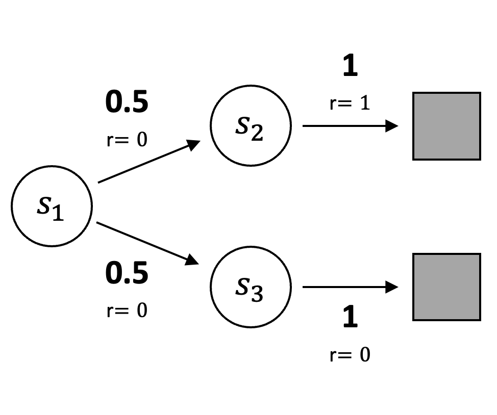Assuming \(\gamma = 1\) and on-policy training (\(\rho = 1\)), the true state values can be analytically computed as: \(V(s_1) = \frac{1}{2}\), \(V(s_2) = 1\), and \(V(s_3) = 0\). However, the values that minimize \(\overline{\text{TDE}}\), \(V(s_1) = \frac{1}{2}\), \(V(s_2) = \frac{3}{4}\), and \(V(s_3) = \frac{1}{4}\), differ from the true values.

To demonstrate this, we compute \(\overline{\text{TDE}}\) for both the minimizing value function and the true value function, starting with the former:

\[ \begin{align*} \overline{\text{TDE}}(s_1 \to s_2) &= \left( 0 + \frac{3}{4} - \frac{1}{2} \right)^2 = \frac{1}{16} \\ \overline{\text{TDE}}(s_1 \to s_3) &= \left( 0 + \frac{1}{4} - \frac{1}{2} \right)^2 = \frac{1}{16} \\ \overline{\text{TDE}}(s_2 \to s_T) &= \left( 1 + 0 - \frac{3}{4} \right)^2 = \frac{1}{16} \\ \overline{\text{TDE}}(s_3 \to s_T) &= \left( 0 + 0 - \frac{1}{4} \right)^2 = \frac{1}{16} \;. \end{align*} \]

The mean \(\overline{\text{TDE}}\) for these values across all transitions is \(\frac{1}{16}\).

\[ \begin{align*} \overline{\text{TDE}}(s_1 \to s_2) &= \left( 0 + 1 - \frac{1}{2} \right)^2 = \frac{1}{4} \\ \overline{\text{TDE}}(s_1 \to s_3) &= \left( 0 + 0 - \frac{1}{2} \right)^2 = \frac{1}{4} \\ \overline{\text{TDE}}(s_2 \to s_T) &= \left( 1 + 0 - 1 \right)^2 = 0 \\ \overline{\text{TDE}}(s_3 \to s_T) &= \left( 0 + 0 - 0 \right)^2 = 0 \;. \end{align*} \]

The mean \(\overline{\text{TDE}}\) for the true values across all transitions is \(\frac{1}{8}\).

Since \(\frac{1}{8} > \frac{1}{16}\), the true values result in a higher \(\overline{\text{TDE}}\). This demonstrates that minimizing \(\overline{\text{TDE}}\) does not necessarily yield the true state values, highlighting a fundamental limitation of this approach.

In contrast to the TD error, the Bellman Error is guaranteed to be zero if the exact values are learned. Thus, minimizing the mean squared Bellman Error, \(\overline{\text{BE}}\), is a seemingly natural objective. Its associated update rule is as follows:

\[ \begin{align} \theta_{t+1} &= \theta_t - \frac{1}{2} \alpha \nabla \left( \mathbb{E}_\pi[ \delta_t ]^2 \right) \nonumber \\ &= \theta_t - \frac{1}{2} \alpha \nabla \left( \mathbb{E}_{\pi_\beta}[ \rho_t \delta_t ]^2 \right) \nonumber \\ &= \theta_t - \alpha \mathbb{E}_{\pi_\beta}[ \rho_t \delta_t ] \nabla \mathbb{E}_{\pi_\beta}[ \rho_t \delta_t ] && \text{by the chain rule} \nonumber \\ &= \theta_t - \alpha \mathbb{E}_{\pi_\beta}[ \rho_t \delta_t ] \, \mathbb{E}_{\pi_\beta}[ \rho_t \nabla \delta_t ] \label{eq:beu-1} \\ &= \theta_t - \alpha \mathbb{E}_{\pi_\beta}[ \rho_t \big( r_{t+1} + \gamma \hat{V}_\theta(s_{t+1}) - \hat{V}_\theta(s_t) \big) ] \mathbb{E}_{\pi_\beta} \left[ \rho_t \nabla \big( r_{t+1} + \gamma \hat{V}_\theta(s_{t+1}) - \hat{V}_\theta(s_t) \big) \right] \label{eq:beu-2} \\ &= \theta_t - \alpha \mathbb{E}_{\pi_\beta}[ \rho_t ( r_{t+1} + \gamma \hat{V}_\theta(s_{t+1}) - \hat{V}_\theta(s_t) ) ] \mathbb{E}_{\pi_\beta}[ \rho_t ( \gamma \nabla \hat{V}_\theta(s_{t+1}) - \nabla \hat{V}_\theta(s_t) ) ] && \text {by the sum rule in differentiation} \label{eq:beu-3} \\ &= \theta_t - \alpha \left( \mathbb{E}_{\pi_\beta}[ \rho_t ( r_{t+1} + \gamma \hat{V}_\theta(s_{t+1}) ) ] - \hat{V}_\theta(s_t) \right) \left( \gamma \mathbb{E}_{\pi_\beta}[ \rho_t \nabla \hat{V}_\theta(s_{t+1}) ] - \nabla \hat{V}_\theta(s_t) \right) \label{eq:beu-4} \\ &= \theta_t + \alpha \left[ \mathbb{E}_{\pi_\beta} \left[ \rho_t \left( r_{t+1} + \gamma \hat{V}_{\theta}(s_{t+1}) \right) \right] - \hat{V}_{\theta}(s_t) \right] \left[ \nabla \hat{V}_{\theta}(s_t) - \gamma \mathbb{E}_{\pi_\beta} \left[ \rho_t \nabla \hat{V}_{\theta}(s_{t+1}) \right] \right] \;. \label{eq:beu-5} \end{align} \]

The transition from Equation \(\eqref{eq:beu-3}\) to Equation \(\eqref{eq:beu-4}\) holds because the expectation \(\mathbb{E}_{\pi_\beta}[\cdot]\) is taken over transitions originating from state \(s_t\). Within this conditional expectation, any term that depends only on \(s_t\) — and not on \(a_t\), \(r_{t+1}\), or \(s_{t+1}\) — is constant with respect to the expectation. Consequently, \(\hat{V}(s_t; \theta_t)\) and \(\nabla \hat{V}(s_t; \theta_t)\) can be factored out of the expectation. The importance sampling ratio \(\rho_t\) is dropped from these terms because the conditional expectation of the \(\rho_t\) at \(s_t\) equals one:

\[ \begin{align*} \mathbb{E}_{\pi_\beta}[\rho_t \mid s_t] &= \mathbb{E}_{\pi_\beta}\!\left[\frac{\pi(a_t \mid s_t)}{\pi_\beta(a_t \mid s_t)} \,\middle|\, s_t\right] \\ &= \sum_{a_t} \pi_\beta(a_t \mid s_t) \frac{\pi(a_t \mid s_t)}{\pi_\beta(a_t \mid s_t)} \\ &= \sum_{a_t} \pi(a_t \mid s_t) \\ &= 1 \;. \end{align*} \]

The update in Equation \(\eqref{eq:beu-5}\), together with the associated sampling methods, is known as the residual-gradient algorithm.

Double Sampling Problem

Equation \(\eqref{eq:beu-1}\) involves the product of two expectations, \(\mathbb{E}[X]\) and \(\mathbb{E}[Y]\), where \(X = \rho_t \delta_t\) and \(Y = \rho_t \nabla \delta_t\). This formulation theoretically leads to the update:

\[ \begin{equation*} \theta_{t+1} = \theta_t - \alpha \mathbb{E}[X] \mathbb{E}[Y] \;. \end{equation*} \]

In practice, however, \(\mathbb{E}[X]\) and \(\mathbb{E}[Y]\) are approximated using sample estimates \(x\) and \(y\), resulting in an update of the form:

\[ \begin{equation*} \theta_{t+1} = \theta_t - \alpha x y \;. \end{equation*} \]

An estimator is unbiased if its expected value equals the true value of the parameter it estimates. For \(x y\), the product of the sample estimates of the random variables \(X\) and \(Y\), to be an unbiased estimator of \(\mathbb{E}[X] \mathbb{E}[Y]\), it must be true that \(\mathbb{E}[X Y] = \mathbb{E}[X] \mathbb{E}[Y]\). This equality holds only when \(x\) and \(y\) are independent. In this update rule, however, \(x\) and \(y\) are dependent, as both are functions of the same underlying sample, \(s_{t+1}\) (as illustrated most clearly beginning in Equation \(\eqref{eq:beu-2}\)). This dependence introduces a bias in the approximation, leading to the double sampling problem.

To address this bias, two independent samples of \(s_{t+1}\) would be required. While this is feasible in simulated environments — where we can roll back to \(s_t\) and simulate alternative next states — it is not generally possible in real-world settings. Alternatively, in deterministic environments, state transitions are fixed, ensuring that any two samples of \(s_{t+1}\) are identical (assuming a deterministic policy). In such cases, Equation \(\eqref{eq:beu-5}\) remains valid, and no rollback procedure is necessary.

Resolving this bias using either of these approaches ensures that any function approximator (linear or nonlinear) using this update rule converges to a minimum of \(\overline{\text{BE}}\), under the usual conditions on the step-size parameter \(\alpha\). In the linear case, convergence is guaranteed to the unique \(\theta\) that minimizes \(\overline{\text{BE}}\). Nonetheless, three significant issues persist: (1) this method is considerably slower than semi-gradient methods, (2) like the TD error, the solution that minimizes the Bellman error is not necessarily the same solution that minimizes the true Value Error, and (3) the Bellman Error is not learnable.

In Practice

Despite the learnability challenges of these objectives and the divergence risks inherent in naive semi-gradient methods, modern deep RL has achieved practical success. Contemporary approaches typically perform semi-gradient descent on the Mean Squared TD Error (TDE) objective, with each update driven by the TD error from a single experience. Stability in off-policy learning is attained not through true-gradient optimization but through techniques such as experience replay and target networks.

References

- Reinforcement Learning: An Introduction (2018)
Richard S. Sutton and Andrew G. Barto
- Residual Algorithms (accessed 2023)
Machine Learning Glossary at Carnegie Mellon University
- Why Should I Trust You, Bellman? The Bellman Error is a Poor Replacement for Value Error (2022)
Scott Fujimoto, David Meger, Doina Precup, Ofir Nachum, and Shixiang Shane Gu
- Borrowing From the Future: An Attempt to Address Double Sampling, Mathematical and scientific machine learning (2020)
Yuhua Zhu and Lexing Ying
- Review of Probability and Stochastic gradient descent (2018)
Courtney Paquette
- If Q-learning is off-policy, why doesn't it require importance sampling? (accessed 2024)
James MacGlashan