PID Lagrangian
Revised August 22, 2025
The Constrained Markov Decision Processes note is optional but recommended background reading.
In primal-dual methods for constrained MDPs, constraints affect the policy optimization only through the Lagrange multipliers:
\[ \begin{equation*} \max_\theta \min_{\lambda \geq 0} \mathcal{L}(\theta, \lambda) = J^\pi(\theta) - \lambda \big(J_c^\pi(\theta) - l\big). \end{equation*} \]
Because the primal and dual updates are coupled, intermediate policies can violate constraints; feasibility is guaranteed only at a saddle point \((\pi^*, \lambda^*)\), where the KKT conditions hold. The PID Lagrangian method mitigates these transient violations by interpreting the dual update as a feedback controller: the multiplier \(\lambda\) regulates the constraint cost around the setpoint \(l\). In this framework, proportional feedback improves responsiveness, integral feedback eliminates steady-state error, and derivative feedback damps fluctuations.
PID Controller
Proportional–Integral–Derivative (PID) control is a fundamental scheme in classical control theory. A PID controller computes the error \(e(t)\) between a desired setpoint and a measured process variable, and adjusts the control input through proportional, integral, and derivative terms. The proportional term applies an output \(K_P e(t)\), scaling the immediate error by the gain \(K_P\). The integral term applies \(K_I \int_0^t e(\tau)\,d\tau\), which accumulates past error to remove steady-state offsets that persist under proportional control alone. Its strength is governed by the integral gain \(K_I\). The derivative term applies \(K_D \tfrac{d}{dt} e(t)\), which reacts to the rate of error change. This anticipatory action improves stability and mitigates overshoot by damping rapid deviations. The derivative gain \(K_D\) sets the magnitude of this effect. Together, these components balance responsiveness, accuracy, and stability. The gains \((K_P, K_I, K_D)\) are typically treated as tunable hyperparameters. Their effects can be summarized as follows:
Proportional Term (\(K_P\))
Higher \(K_P\): Increases responsiveness to error, reducing constraint violations more quickly. Excessive values induce oversensitivity, instability, or oscillations.
Lower \(K_P\): Slows error correction and may yield inadequate responses.
Integral Term (\(K_I\))
Higher \(K_I\): Eliminates steady-state error by correcting accumulated bias. Excessive values amplify oscillations and slow convergence due to large corrective swings.
Lower \(K_I\): Weakens correction of persistent error, allowing steady-state deviations to remain.
Derivative Term (\(K_D\))
Higher \(K_D\): Provides anticipatory damping based on the error's rate of change, reducing overshoot and improving stability. Excessive values cause aggressive reactions to error fluctuations, destabilizing the system.
Lower \(K_D\): Diminishes damping, leading to overshoot and less stable responses.
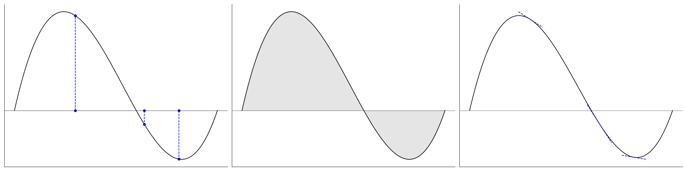 |
| This figure illustrates the contribution of each term in PID control. The x-axis denotes timesteps and the y-axis the constraint function value. The black curve represents the constraint trajectory, and the horizontal gray line marks the constraint limit. The proportional term (left) depends only on the instantaneous deviation at each timestep. The integral term (middle) accumulates deviations over time, so even a small but persistent violation eventually produces a substantial corrective effect. The derivative term (right) responds to the rate of change of the constraint, damping rapid deviations before they can accumulate. |
Constraint-Controlled Reinforcement Learning
The dual update in the standard Lagrangian formulation:
\[ \begin{align*} \nabla_\theta \mathcal{L}(\theta, \lambda) &= \nabla_\theta J^\pi(\theta) - \lambda \nabla_\theta J_c^\pi(\theta), \\ \nabla_\lambda \mathcal{L}(\theta, \lambda) &= -\left(J_c^\pi(\theta) - l \right) \;, \end{align*} \]
is equivalent to an integral-only controller, where the learning rate \(\alpha_\lambda\) serves as \(K_I\). The multiplier \(\lambda\) accumulates deviations of the constraint cost \(J_c^\pi\) from the limit \(l\). Proportional and derivative corrections can be incorporated by augmenting the update with additional feedback terms:
\[ \begin{equation}\label{eq:pid-multiplier} \lambda_{t+1} = \Big[ K_P \big(J_c^\pi(\theta_t) - l\big) + K_I \sum_{\tau=0}^t \big(J_c^\pi(\theta_\tau) - l\big) + K_D \big(J_c^\pi(\theta_t) - J_c^\pi(\theta_{t-1})\big)_+ \Big]_+ \;. \end{equation} \]
The operator \((x)_+\) denotes the positive part, defined as \(\max\{x,0\}\). It is applied to \((J_c^\pi(\theta_t)-J_c^\pi(\theta_{t-1}))\) so that the derivative term responds only to increases in violation, and in the projection step \([\cdot]_+\) to enforce \(\lambda_{t+1}\ge 0\). Equation \(\eqref{eq:pid-multiplier}\) can be expressed as an update rule as follows:
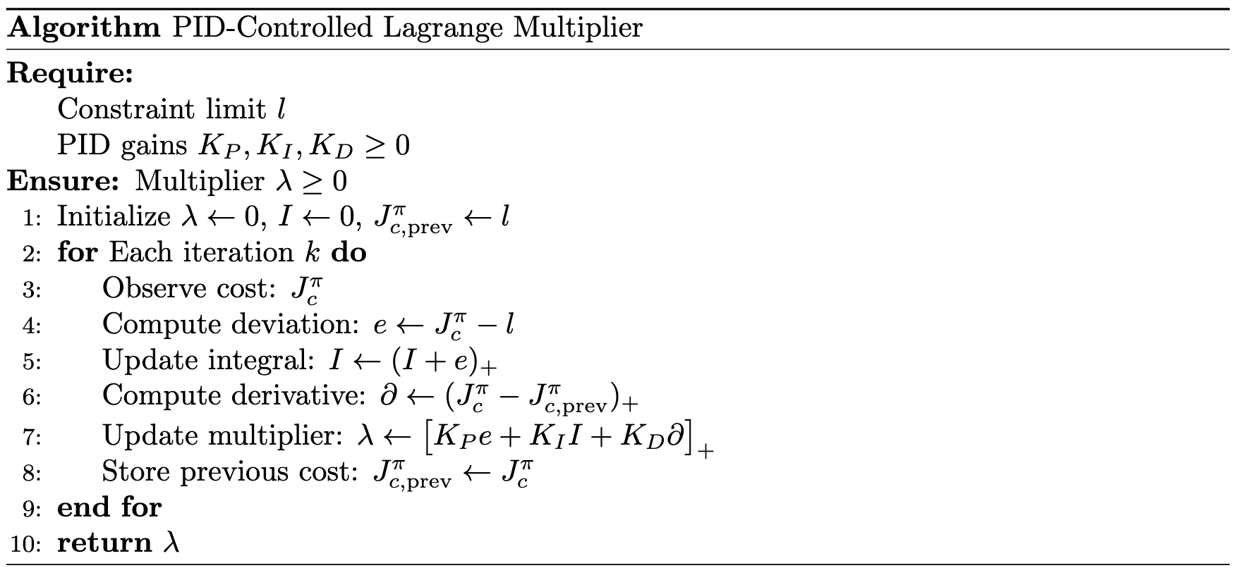 |
This PID update defines a dynamical system for the multiplier. In practice, it is embedded directly within a reinforcement learning scheme (e.g., PPO):
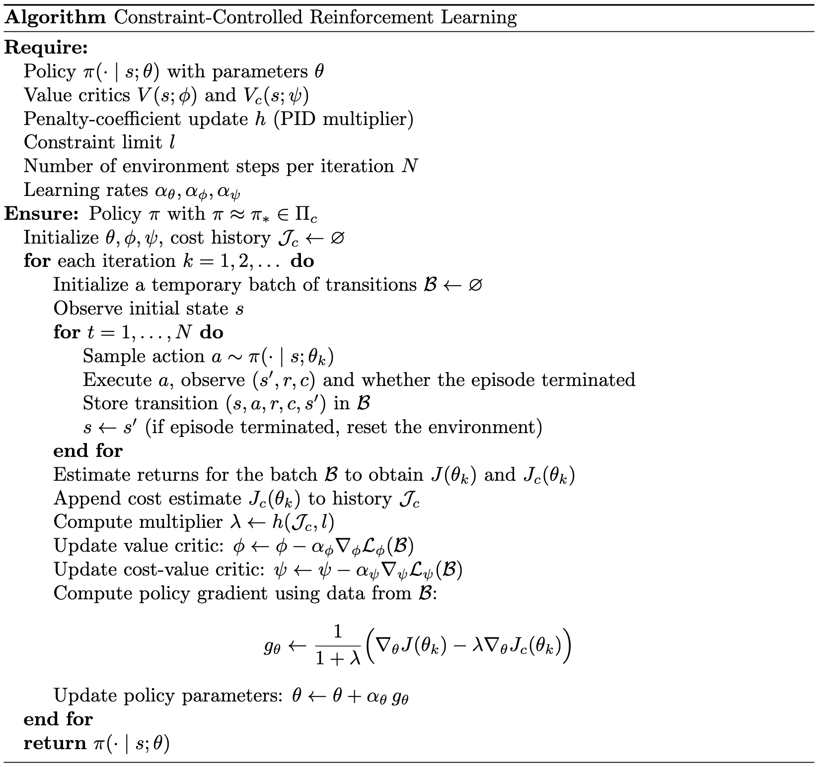 |
The approach employs two mechanisms to stabilize updates under a varying penalty coefficient \(\lambda\). First, it separates value and cost-value critics to prevent interference between reward and cost signals, reducing instability when \(\lambda\) changes rapidly. Second, it rescales the policy gradient:
\[ \begin{equation*} \mathcal{L}(\theta;\lambda) = J(\theta) - \lambda J_c(\theta), \end{equation*} \]
to offset the large parameter updates induced when \(\lambda\) heavily weights the cost term in the penalized objective, giving the modified gradient:
\[ \begin{equation*} \nabla_\theta \mathcal{L}(\theta;\lambda) = \frac{1}{1+\lambda}\Big(\nabla_\theta J(\theta) - \lambda \nabla_\theta J_c(\theta)\Big) \;. \end{equation*} \]
Improving Robustness Within and Across Environments
Consider two CMDPs that are identical except the rewards in one are scaled by a constant \(\rho\). Then \(J\) and \(\nabla_\theta J\) scale by \(\rho\) while \(J_c\) and \(\nabla_\theta J_c\) remain unchanged. To preserve the Lagrangian tradeoff \(J - \lambda J_c\) and the resulting learning dynamics, the optimal rescales as \(\lambda^* \mapsto \rho\,\lambda^*\). For the standard (unnormalized) Lagrangian update, this implies that the controller parameters must also scale: \(\lambda_0 \mapsto \rho \lambda_0\) and \((K_P, K_I, K_D) \mapsto \rho (K_P, K_I, K_D)\). To avoid this sensitivity to the reward scale, we instead use the normalized update
\[ \begin{equation*} \nabla_\theta \mathcal{L} = (1 - u_k)\,\nabla_\theta J^\pi(\theta_k) - u_k\,\beta_k\,\nabla_\theta J_c^\pi(\theta_k) \;, \end{equation*} \]
where \(0 \leq u_k = \lambda_k/(1+\lambda_k) \leq 1\). With this normalization, \(\lambda\) retains a consistent operational meaning independent of reward scaling. The ratio of unscaled policy gradients is a natural choice for \(\beta_k\):
\[ \begin{equation*} \beta_{\nabla, k} = \frac{\| \nabla_\theta J(\theta_k) \|}{\| \nabla_\theta J_c(\theta_k) \|} \;. \end{equation*} \]
When \(\lambda=1\), the reward and cost gradients are scaled to have equal norm, so the update is balanced and \(\lambda\) directly controls their relative weighting.
Citation
Landers, Matthew. "PID Lagrangian." mattlanders.net, August 22, 2025. mattlanders.net/pid-lagrangian.
@article{landers2025pid,
  title = {PID Lagrangian},
  author = {Landers, Matthew},
  journal = {mattlanders.net},
  year = {2025},
  month = {August},
  url = "mattlanders.net/pid-lagrangian"
}
References
- Responsive Safety in Reinforcement Learning by PID Lagrangian Methods, International Conference on Machine Learning (2020)
Adam Stooke, Joshua Achiam, and Pieter Abbeel
- Benchmarking Safe Exploration in Deep Reinforcement Learning (2019)
Alex Ray, Joshua Achiam, and Dario Amodei
- PID Control - A brief introduction [video] (2013)
Brian Douglas