Kullback–Leibler (KL) Divergence
Revised September 2, 2025
The Importance Sampling note is optional but recommended background reading.
Importance sampling expresses the return of a target policy \(\pi\) using trajectories generated by a behavior policy \(\mu\):
\[ \begin{equation*} \mathbb{E}_{\tau \sim p_\pi}[G(\tau)] = \mathbb{E}_{\tau \sim p_\mu}\!\left[\frac{p_\pi(\tau)}{p_\mu(\tau)}\,G(\tau)\right]. \end{equation*} \]
where \(\tau=(s_0,a_0,\dots,s_{T-1},s_T)\) and \(p_\pi(\tau)=\rho_0(s_0)\prod_{t=0}^{T-1}\pi(a_t\mid s_t)\,P(s_{t+1}\mid s_t,a_t)\) with the same \(\rho_0\) and \(P\) for \(\pi\) and \(\mu\).
The importance weight for a trajectory factorizes into a product of per-step action probabilities:
\[ \begin{equation*} \frac{p_\pi(\tau)}{p_\mu(\tau)} = \prod_{t=0}^{T-1} \frac{\pi(a_t\mid s_t)}{\mu(a_t\mid s_t)}. \end{equation*} \]
This product has high variance when \(\pi\) and \(\mu\) differ substantially. Moreover, its multiplicative structure is numerically unstable and obscures the contribution of individual decisions. Applying a logarithm converts products into sums, yielding a per-step additive form:
\[ \begin{equation*} \log \frac{p_\pi(\tau)}{p_\mu(\tau)} = \sum_{t=0}^{T-1} \log \frac{\pi(a_t\mid s_t)}{\mu(a_t\mid s_t)} \;. \end{equation*} \]
This decomposition is more stable and isolates the influence of each action on the total ratio. Averaging this quantity under \(p_\pi\) produces:
\[ \begin{equation*} \mathbb{E}_{\tau \sim p_\pi}\!\left[ \log \frac{p_\pi(\tau)}{p_\mu(\tau)} \right], \end{equation*} \]
which defines the Kullback–Leibler (KL) divergence:
\[ \begin{equation}\label{eq:kl-divergence} D_{KL}(p_\pi \,\Vert\, p_\mu) = \mathbb{E}_{\tau \sim p_\pi}\!\left[ \log \frac{p_\pi(\tau)}{p_\mu(\tau)} \right] \;. \end{equation} \]
Importance sampling fails when \(\pi(a\mid s)>0\) but \(\mu(a\mid s)=0\), since the ratio \(\tfrac{\pi(a\mid s)}{\mu(a\mid s)}\) is undefined. More generally, stable estimates require the per-step ratios \(\tfrac{\pi(\cdot\mid s)}{\mu(\cdot\mid s)}\) to remain near one on the support of \(d_\pi\), the discounted state visitation distribution under \(\pi\). This condition corresponds to a small KL divergence between \(p_\pi\) and \(p_\mu\). TRPO constrains the expected per-state KL between the new and old policy under the old state distribution; PPO achieves a similar effect via clipping.
In maximum-entropy reinforcement learning such as SAC, KL divergence acts as a projection onto \(P_{\text{opt}}\), the distribution over optimal trajectories. Minimizing \(D_{KL}(p_\pi \,\Vert\, P_{\text{opt}})\) shifts probability mass toward high-return trajectories:
\[ \begin{align} D_{KL}(p_\pi \Vert P_{\text{opt}}) &= \mathbb{E}_{\tau \sim p_\pi}\!\left[\log p_\pi(\tau) - \log P_{\text{opt}}(\tau)\right] && \text{by Equation } \eqref{eq:kl-divergence} \label{eq:entropy-kl} \\ &= \mathbb{E}_{\tau \sim p_\pi}[\log p_\pi(\tau)] - \mathbb{E}_{\tau \sim p_\pi} \left[ \tfrac{1}{\alpha}\sum_t \gamma^t r(s_t,a_t) - \log Z \right] && \text{with } P_{\text{opt}}(\tau)=\tfrac{1}{Z}\exp\!\Big(\tfrac{1}{\alpha}\sum_t \gamma^t r(s_t,a_t)\Big) \nonumber \\ &= -H(p_\pi) - \tfrac{1}{\alpha}\mathbb{E}_{\tau \sim p_\pi}\!\Big[\sum_t \gamma^t r(s_t,a_t)\Big] + \log Z && \text{where } H(p_\pi) = -\,\mathbb{E}_{\tau \sim p_\pi}[\log p_\pi(\tau)] \nonumber \end{align} \]
Since \(\log Z\) and \(\alpha\) are constant with respect to \(\pi\), minimizing Equation \(\eqref{eq:entropy-kl}\) is equivalent to maximizing:
\[ \begin{equation*} \mathbb{E}_{\tau \sim p_\pi}\!\Big[\sum_{t=0}^{T-1} \gamma^t r(s_t,a_t)\Big] + \alpha H(p_\pi) \;, \end{equation*} \]
which coincides with the maximum-entropy reinforcement learning objective.
Equation \(\eqref{eq:kl-divergence}\), the reverse KL divergence, tends to be mode-seeking. Because the expectation is taken under \(p_\pi\), regions where \(p_\pi(\tau)=0\) contribute nothing even if \(p_\mu(\tau)\) is large, while placing mass where \(p_\mu(\tau)\approx 0\) incurs an infinite (or very large) penalty. This asymmetry encourages \(p_\pi\) to concentrate on one (or a few) high-probability modes of \(p_\mu\) rather than spreading mass across all modes. This behavior is consistent with RL in fully observed MDPs with an expected-return objective, where there exists an optimal deterministic policy that concentrates on \(\arg\max_a Q^*(s,a)\) (though stochastic optima can arise with ties, partial observability, or explicit regularization).
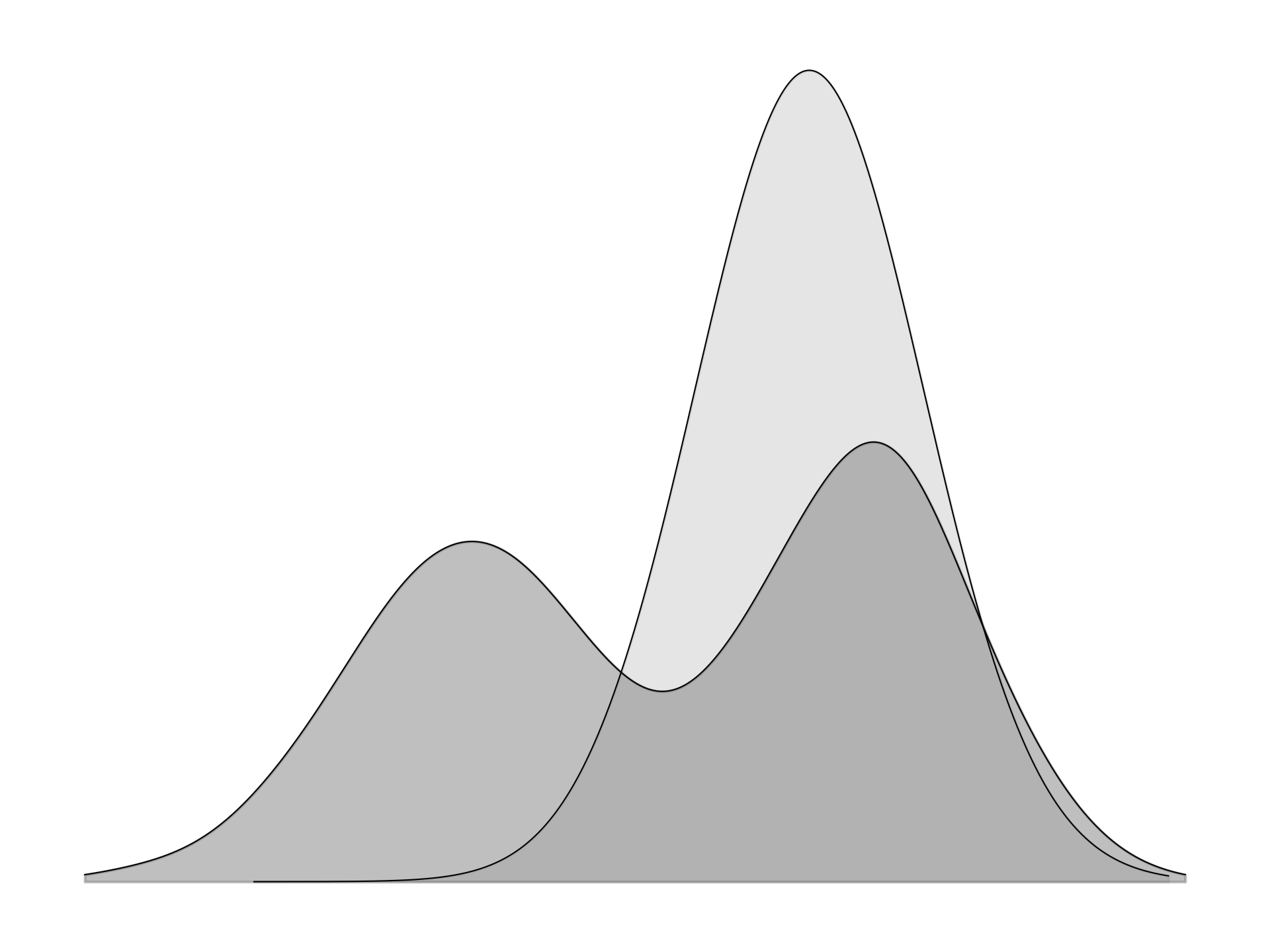 |
| \(p_\mu\) is a bimodal distribution and \(p_\pi\) is a Gaussian approximation. Reverse KL places mass on a single mode of \(p_\mu\). |
Forward KL Divergence
Reverse KL divergence is natural in policy optimization, since expectations are taken under the policy \(p_\pi\), which can be sampled directly. In supervised learning, by contrast, samples from the data distribution \(p_\mu\) are available, but its density is unknown. A parametric model \(p_\pi\) is therefore introduced to approximate \(p_\mu\), leading to the forward KL divergence, where the expectation in Equation \(\eqref{eq:kl-divergence}\) is taken with respect to \(p_\mu\):
\[ \begin{equation}\label{eq:forward-kl} D_{KL}(p_\mu \,\Vert\, p_\pi) = \mathbb{E}_{\color{red}{\tau \sim p_\mu}} \left[ \log \frac{p_\mu(\tau)}{p_\pi(\tau)} \right] \;. \end{equation} \]
Terms with \(p_\mu(\tau)=0\) vanish, so only regions where \(p_\mu\) has support contribute. Forward KL divergence thus penalizes \(p_\pi\) for assigning low probability where \(p_\mu\) is positive, but not for placing mass where \(p_\mu\) is zero. Minimization therefore requires \(p_\pi\) to cover the full support of \(p_\mu\).
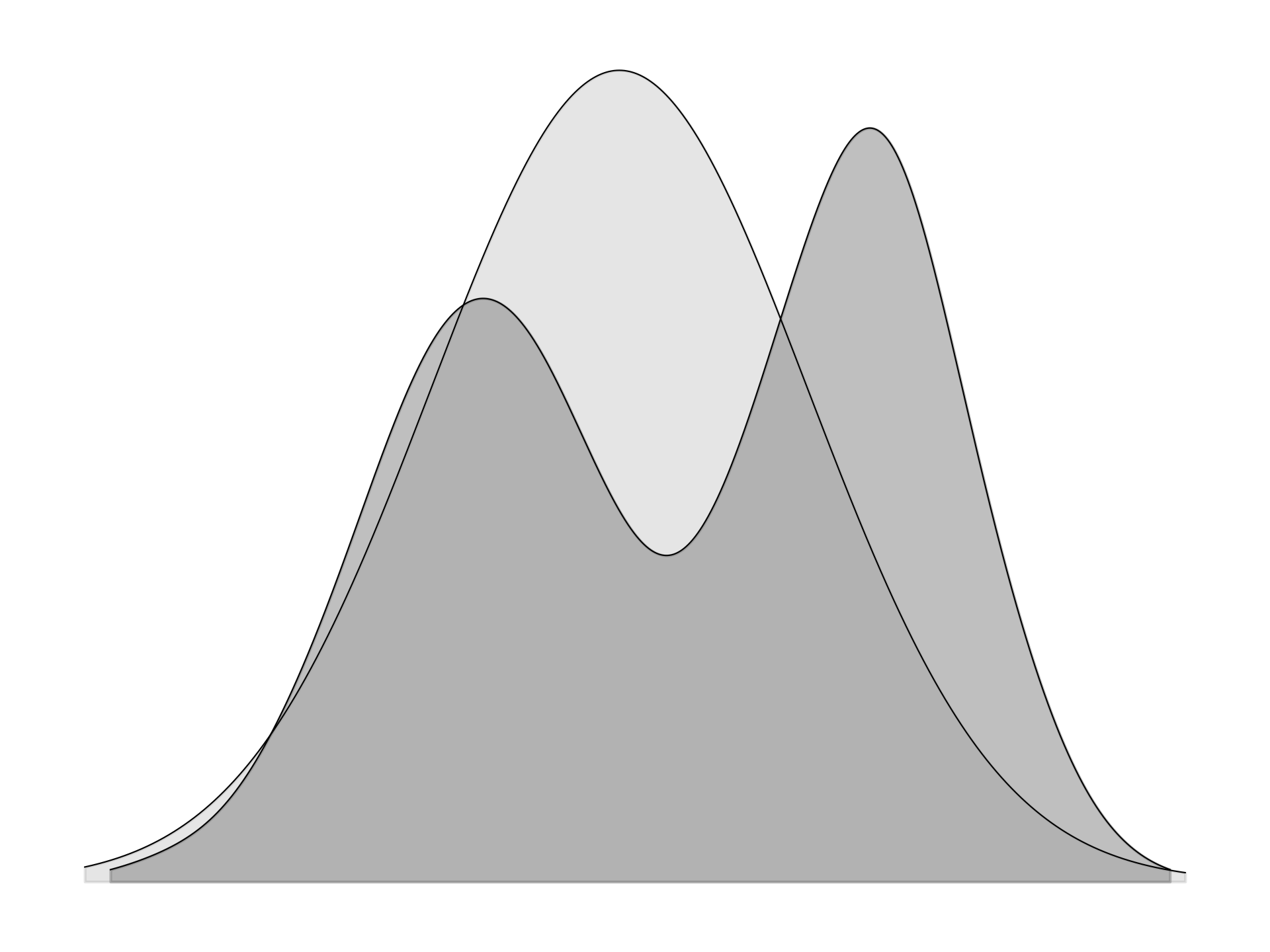 |
| \(p_\mu\) is a bimodal distribution and \(p_\pi\) is a Gaussian approximation. Because \(p_\pi\) must spread mass across the support of \(p_\mu\), forward KL divergence is characterized as mean-seeking. |
Forward KL coincides with maximum likelihood estimation, which provides the statistical foundation for standard supervised learning objectives. Given samples from the data distribution \(p_\mu\), a parametric model \(p_\pi\) is chosen to minimize \(D_{KL}(p_\mu \Vert p_\pi)\):
\[ \begin{align*} D_{KL}(p_\mu \Vert p_\pi) &= \mathbb{E}_{x \sim p_\mu}\!\left[\log p_\mu(x) - \log p_\pi(x)\right] && \text{by Equation } \eqref{eq:forward-kl} \\ &= \mathbb{E}_{x \sim p_\mu}\!\left[\log p_\mu(x)\right] - \mathbb{E}_{x \sim p_\mu}\!\left[\log p_\pi(x)\right] && \text{linearity of expectation} \\ &= -\mathbb{E}_{x \sim p_\mu}[\log p_\pi(x)] - H(p_\mu) && \text{definition of Shannon entropy.} \end{align*} \]
The entropy term \(H(p_\mu)\) is independent of \(\pi\), so minimizing forward KL divergence is equivalent to maximizing the log-likelihood of the data under \(p_\pi\).
For classification, let \(p_\pi(y\mid x)\) be the categorical distribution defined by \(f_\pi(x)\). The cross-entropy loss:
\[ \begin{equation*} \mathcal{L}_{\text{CE}} = \mathbb{E}_{(x,y)\sim p_\mu}\!\big[-\log p_\pi(y\mid x)\big] \end{equation*} \]
differs from \(D_{KL}(p_\mu\Vert p_\pi)\) only by the constant \(H(p_\mu)\). Minimizing cross-entropy is therefore equivalent to minimizing forward KL.
For regression, if \(p_\pi(y\mid x)\) is Gaussian with mean \(f_\pi(x)\) and fixed variance, then:
\[ \begin{equation*} -\log p_\pi(y\mid x)=\tfrac{1}{2\sigma^2}|y-f_\pi(x)|_2^2 + C \end{equation*} \]
for fixed variance \(\sigma^2\). Thus, minimizing mean squared error coincides with forward KL under the Gaussian model. Both cross-entropy (classification) and squared error (regression) are therefore special cases of forward KL minimization.
Citation
Landers, Matthew. "Kullback–Leibler (KL) Divergence." mattlanders.net, September 2, 2025. mattlanders.net/kl-divergence.
@article{landers2025kullbackleibler,
  title = {Kullback–Leibler (KL) Divergence},
  author = {Landers, Matthew},
  journal = {mattlanders.net},
  year = {2025},
  month = {September},
  url = "mattlanders.net/kl-divergence"
}
References
- KL Divergence for Machine Learning (2018)
Dibya Ghosh
- Demystifying Entropy (And More) (2019)
Jake Tae
- Six (and a half) intuitions for KL divergence (2022)
Callum McDougall