On-Policy Control with Function Approximation
Revised November 4, 2024
The Model-Free Control note is optional but recommended background reading.
Control with function approximation requires distinct treatment of on-policy and off-policy approaches, as tabular methods extend more naturally to the on-policy domain. This note focuses exclusively on on-policy methods, where despite parallels with tabular control, theoretical distinctions arise. Most notably, while episodic tasks allow for straightforward generalization of tabular methods, continuing tasks require a fundamental reexamination of discounting's role in defining optimal policies.
Episodic Tasks
In prediction with function approximation, we use stochastic gradient descent (SGD) to find the weight vector \(\theta\) that minimizes mean squared error between the approximate state-value function \(\hat{V}(\theta)\) and the true state-value function \(V_\pi\). This approach extends naturally to episodic control with function approximation, with one key distinction: since control methods evaluate state-action pairs, the update target includes the state-action value function \(Q_\pi(s_t,a_t)\). It thus follows that the SGD update for episodic control closely resembles the prediction update, only replacing \(\hat{V}(\theta)\) with \(\hat{Q}(\theta)\):
\[ \begin{equation*} \theta_{t+1} = \theta_t + \alpha \left[ r_{t+1} + \gamma \hat{Q}(s_{t+1}, a_{t+1}; \theta_t) - \hat{Q}(s_t, a_t; \theta_t) \right] \nabla \hat{Q}(s_t, a_t; \theta_t) \;. \end{equation*} \]
To estimate the optimal action-value function \(Q_*\), we can reuse our tabular algorithms with small modifications. In semi-gradient SARSA, for example, we determine the greedy action \(a_{t+1}^* = \text{arg}\max_{a} \hat{Q}(s_{t+1}, a; \theta_t)\) by evaluating \(\hat{Q}(s_{t+1}, a; \theta_t)\) for all possible actions \(a\) in state \(s_{t+1}\), followed by \(\epsilon\)-greedy action selection for policy improvement:
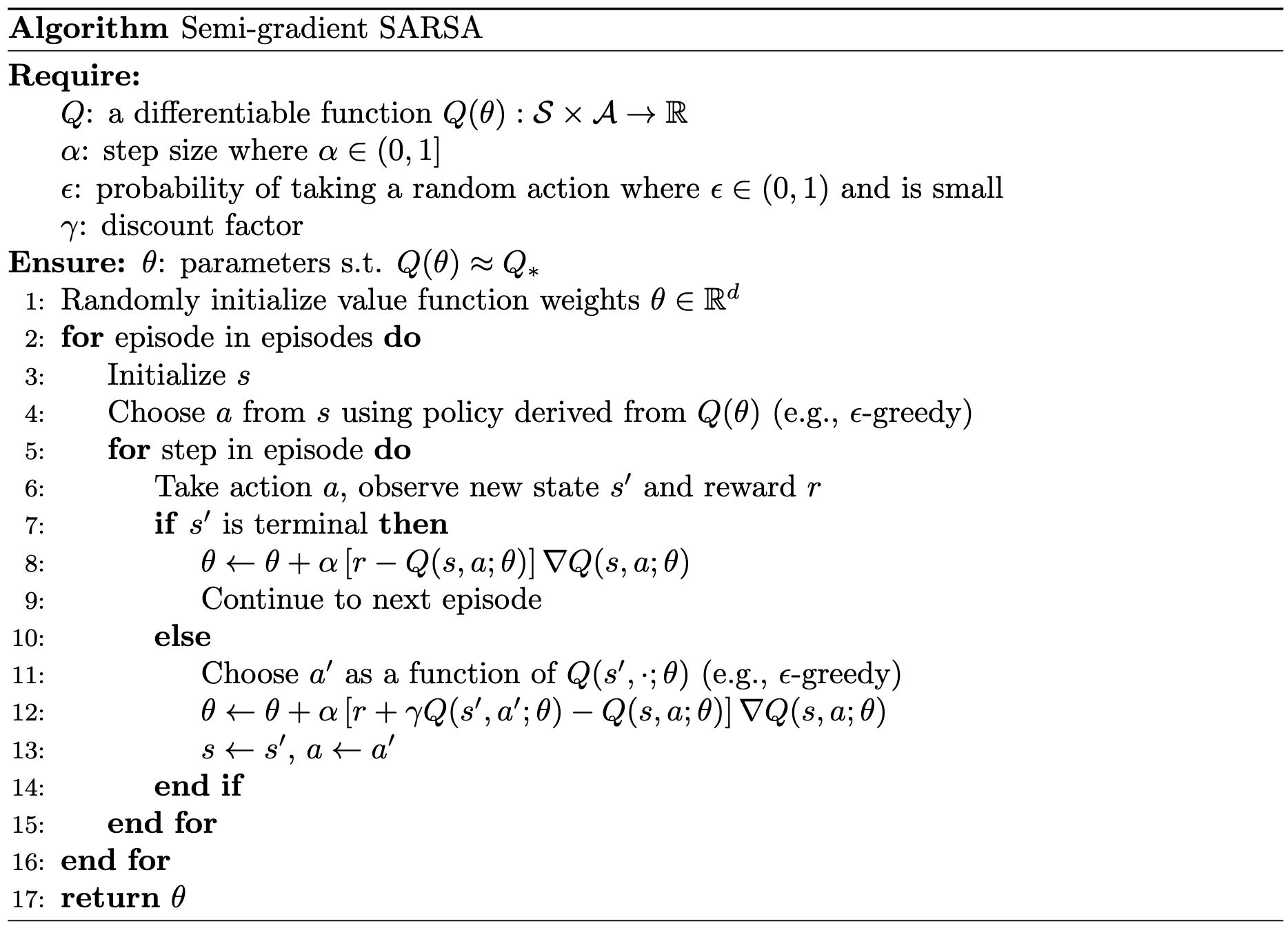 |
This approach, while effective, necessitates discrete and manageable action spaces due to the exhaustive evaluation of actions in \(s_{t+1}\). For continuous or large discrete action spaces, more sophisticated techniques are necessary.
Continuing Tasks
In continuing tasks with function approximation, returns are defined in terms of average rewards rather than the typical discounted rewards.
\[ \begin{align} R(\pi) &= \lim_{H \rightarrow \infty} \frac{1}{H} \sum_{t=1}^H \mathbb{E} \left[ r_t \mid s_0, a_{0:t-1} \sim \pi \right] \label{eq:ar1} \\ &= \lim_{t \rightarrow \infty} \mathbb{E} \left[ r_t \mid s_0, a_{0:t-1} \sim \pi \right] \label{eq:ar2} \\ &= \sum_s \mu_\pi(s) \sum_a \pi(a \mid s) R(s,a) \;, \label{eq:ar3} \end{align} \]
where \(H\) is the horizon length, \(\mu_\pi(s)\) is the on-policy distribution, and the expectations are computed given the initial state \(s_0\) and the sequence of actions \(a_{0:t-1} = a_0, a_1, \dots, a_{t-1}\) generated by policy \(\pi\).
The equivalence of Equation \(\eqref{eq:ar2}\) and Equation \(\eqref{eq:ar3}\) holds when the MDP is ergodic, meaning a steady-state distribution:
\[ \begin{equation}\label{eq:ss-dist} \sum_s \mu_\pi(s) \sum_a \pi(a \mid s) P(s’ \mid s,a) = \mu_\pi(s’) \;, \end{equation} \]
exists and is independent of \(s_0\). In an ergodic MDP, the influence of the initial state and early actions diminishes over time. Thus, in the long run, the likelihood of being in any given state depends only on the policy \(\pi\) and the MDP's transition dynamics. This characteristic ensures that the average reward formulation accurately captures the expected behavior of the system as the horizon tends towards infinity.
When using average rewards, we redefine returns in terms of the differential return, which represents the cumulative difference between individual rewards and the average reward:
\[ \begin{align*} G_t &= r_{t+1} - R(\pi) + r_{t+2} - R(\pi) + \cdots \\ &= \sum_{k=0}^\infty \left( r_{t+k+1} - R(\pi) \right) \;. \end{align*} \]
Although this formulation differs from discounted returns, the Bellman equations retain their structure, with only minor adjustments: the discount factor \(\gamma\) is eliminated, and raw rewards are replaced by their deviation from the true average reward. For instance, the action-value Bellman expectation equation and action-value Bellman optimality equation function now takes the form:
\[ \begin{equation*} Q_\pi(s, a) = R(s, a) - R(\pi) + \sum_{s’ \in \mathcal{S}} P(s, a, s’) \left( \sum_{a’ \in \mathcal{A}} \pi(a’ \mid s’) Q_\pi(s’, a’) \right) \\ \;. \end{equation*} \]
and
\[ \begin{equation*} Q_*(s, a) = R(s, a) - \max_\pi R(\pi) + \sum_{s’ \in \mathcal{S}} P(s, a, s’) \max_{a’} Q_*(s’, a’) \;, \end{equation*} \]
respectively.
This change is also reflected in the TD error:
\[ \begin{equation}\label{eq:differential-td} \delta_t = r_{t+1} - \hat{R}_t(\pi) + \hat{Q}(s_{t+1}, a_{t+1}; \theta_t) - \hat{Q}(s_t, a_t; \theta_t) \;, \end{equation} \]
where \(\hat{R}_t(\pi)\) is the estimated average reward \(R(\pi)\) at time \(t\).
In the average reward setting, we can retain the structure of our semi-gradient SARSA algorithm by simply substituting the standard TD error with the differential version:
\[ \begin{equation*} \theta_{t+1} = \theta_t + \alpha \delta_t \nabla \hat{Q}(s_t, a_t; \theta_t) \;, \end{equation*} \]
with \(\delta_t\) given by Equation \(\eqref{eq:differential-td}\).
Discounted rewards are replaced by average rewards in this setting because continuing tasks lack a definitive “beginning” or “end”; they are infinite, with no terminal states to define fixed reference points. As a result, agent performance can only be evaluated through the temporal sequences of rewards and actions, naturally leading to the averaging approach formalized in Equation \(\eqref{eq:ar1}\). While discounting can technically be applied to the average reward, the average of discounted rewards is strictly proportional to the non-discounted average reward \(R(\pi)/(1 - \gamma)\). This proportionality can be demonstrated as follows:
\[ \begin{align*} J(\pi) &= \sum_s \mu_\pi(s) V_\pi^\gamma(s) && \text{where } V_\pi^\gamma \text{ is the discounted value function} \\ &= \sum_s \mu_\pi(s) \sum_a \pi(a \mid s) \left[ R(s, a) + \gamma \sum_{s’} P(s’ \mid s, a) V_\pi^\gamma(s’) \right] && \text{Bellman equation} \\ &= \sum_s \mu_\pi(s) \sum_a \pi(a \mid s) R(s, a) + \gamma \sum_s \mu_\pi(s) \sum_a \pi(a \mid s) \sum_{s’} P(s’ \mid s, a) V_\pi^\gamma(s’) && \text{distributing terms} \\ &= R(\pi) + \gamma \sum_{s’} V_\pi^\gamma(s’) \sum_s \mu_\pi(s) \sum_a \pi(a \mid s) P(s’ \mid s, a) && \text{by Equation \eqref{eq:ar3}} \\ &= R(\pi) + \gamma \sum_{s’} V_\pi^\gamma(s’) \mu_\pi(s’) && \text{by Equation } \eqref{eq:ss-dist} \\ &= R(\pi) + \gamma J(\pi) && \text{by definition of } J(\pi) \;. \end{align*} \]
From here, we solve for \(J(\pi)\) algebraically:
\[ \begin{align*} J(\pi) &= R(\pi) + \gamma J(\pi) \\ J(\pi) - \gamma J(\pi) &= R(\pi) \\ (1 - \gamma) J(\pi) &= R(\pi) \\ J(\pi) &= \frac{1}{1 - \gamma} R(\pi) \;. \end{align*} \]
Thus, for any \(\gamma \in [0,1)\), the relative ranking of policies under the average discounted formulation is identical to that under the average-reward formulation, since the objectives differ only by a scaling factor.
Citation
Landers, Matthew. "On-Policy Control with Function Approximation." mattlanders.net, November 4, 2024. mattlanders.net/on-policy-control-with-function-approximation.
@article{landers2024onpolicy,
  title = {On-Policy Control with Function Approximation},
  author = {Landers, Matthew},
  journal = {mattlanders.net},
  year = {2024},
  month = {November},
  url = "mattlanders.net/on-policy-control-with-function-approximation"
}
References
- Reinforcement Learning: An Introduction (2018)
Richard S. Sutton and Andrew G. Barto
- Reinforcement Learning in Continuous Action Spaces through Sequential Monte Carlo Methods (2007)
Alessandro Lazaric, Marcello Restelli, and Andrea Bonarini
- Application of Newton's Method to action selection in continuous state-and action-space reinforcement learning (2014)
Barry D. Nichols and Dimitris C. Dracopoulos